Day 09: Calculus for Machine Learning

📑 Table of Contents

1. 🌟 Welcome to Day 9
2. 📚 Introduction to Calculus in Machine Learning
   • Why Calculus?
   • Overview of Key Calculus Concepts
   • Installing Necessary Libraries
3. 🧩 Core Concepts
   • Limits and Continuity
   • Derivatives
     • Understanding Derivatives
     • Rules of Differentiation
     • Partial Derivatives
   • Integrals
     • Definite and Indefinite Integrals
     • Applications of Integrals
   • Multivariable Calculus
     • Gradient Vectors
     • Jacobian and Hessian Matrices
   • Optimization Techniques
     • Gradient Descent
     • Stochastic Gradient Descent
4. 💻 Hands-On Coding
   • Example Scripts
5. 🧩 Interactive Exercises
6. 📚 Resources
7. 💡 Tips and Tricks
8. 💡 Best Practices
9. 💡 Advanced Topics
10. 💡 Real-World Applications
11. 💡 Machine Learning Integration
12. 💡 Conclusion

1. 🌟 Welcome to Day 9

Welcome to Day 9 of "Becoming a TensorFlow Boss in 90 Days"! 🎉 Today, we embark on the essential journey of Calculus for Machine Learning. Calculus forms the backbone of many machine learning algorithms, especially those involving optimization and training models. Whether you're fine-tuning neural networks or understanding the mechanics of gradient descent, a solid grasp of calculus is indispensable. By the end of today, you'll have a foundational understanding of key calculus concepts and their practical applications in machine learning. Let’s dive in! 🚀

2. 📚 Introduction to Calculus in Machine Learning

Why Calculus?

Calculus, the mathematical study of continuous change, is pivotal in machine learning for several reasons:

• Optimization: Most machine learning algorithms involve optimizing a loss function to improve model accuracy. Calculus provides the tools to find minima and maxima of these functions.
• Understanding Model Behavior: Concepts like gradients help in comprehending how changes in input features affect the output.
• Backpropagation in Neural Networks: Calculus is fundamental in deriving the backpropagation algorithm, which updates model weights to minimize loss.
• Probabilistic Models: Integrals are used in calculating probabilities and expectations in models like Bayesian networks.

Overview of Key Calculus Concepts

• Limits and Continuity: Foundation for understanding how functions behave as inputs approach certain values.
• Derivatives: Measure the rate at which a function's output changes relative to changes in inputs.
• Partial Derivatives: Extend the concept of derivatives to functions with multiple variables.
• Integrals: Represent the accumulation of quantities and are essential in areas like probability.
• Multivariable Calculus: Deals with functions of multiple variables, crucial for handling high-dimensional data in machine learning.
• Optimization Techniques: Methods like gradient descent rely heavily on calculus to find optimal solutions.

Installing Necessary Libraries

To visualize calculus concepts and perform computations, you'll use NumPy and Matplotlib. If you haven't installed them yet, do so using pip or conda:

pip install numpy matplotlib

Or with Anaconda:

conda install numpy matplotlib

Additionally, SymPy can be useful for symbolic mathematics:

pip install sympy

Or with Anaconda:

conda install sympy

3. 🧩 Core Concepts

🔵 Limits and Continuity

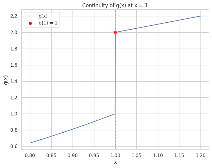
Continuity: A function is continuous at a point if the limit exists and equals the function's value at that point.

import numpy as np
import matplotlib.pyplot as plt

# Define a piecewise function
def g(x):
    if x < 1:
        return x**2
    elif x == 1:
        return 2
    else:
        return x + 1

x = np.linspace(0.8, 1.2, 400)
y = [g(i) for i in x]

plt.figure(figsize=(8, 6))
plt.plot(x, y, label='g(x)')
plt.scatter(1, g(1), color='red', label='g(1) = 2')
plt.title("Continuity of g(x) at x = 1")
plt.xlabel("x")
plt.ylabel("g(x)")
plt.axvline(x=1, color='grey', linestyle='--')
plt.legend()
plt.grid(True)
plt.show()

Output:

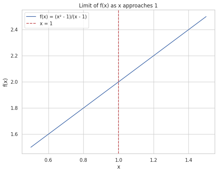
Limit: The value that a function approaches as the input approaches some point.

import numpy as np
import matplotlib.pyplot as plt

# Define a function f(x) = (x^2 - 1)/(x - 1)
def f(x):
    return (x**2 - 1)/(x - 1)

x = np.linspace(0.5, 1.5, 400)
y = f(x)

plt.figure(figsize=(8, 6))
plt.plot(x, y, label='f(x) = (x² - 1)/(x - 1)')
plt.title("Limit of f(x) as x approaches 1")
plt.xlabel("x")
plt.ylabel("f(x)")
plt.axvline(x=1, color='r', linestyle='--', label='x = 1')
plt.legend()
plt.grid(True)
plt.show()

Output:

🟢 Derivatives

📈 Understanding Derivatives

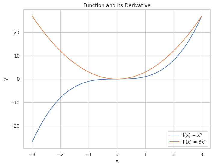
Derivative: Represents the rate of change of a function with respect to a variable.

import numpy as np
import matplotlib.pyplot as plt

# Define a function f(x) = x^3
def f(x):
    return x**3

# Define its derivative f'(x) = 3x^2
def df(x):
    return 3 * x**2

x = np.linspace(-3, 3, 400)
y = f(x)
dy = df(x)

plt.figure(figsize=(8, 6))
plt.plot(x, y, label='f(x) = x³')
plt.plot(x, dy, label="f'(x) = 3x²")
plt.title("Function and Its Derivative")
plt.xlabel("x")
plt.ylabel("y")
plt.legend()
plt.grid(True)
plt.show()

Output:

📉 Rules of Differentiation

• Power Rule: d/dx [x^n] = n * x^(n-1)
• Product Rule: d/dx [u*v] = u'v + uv'
• Quotient Rule: d/dx [u/v] = (u'v - uv') / v²

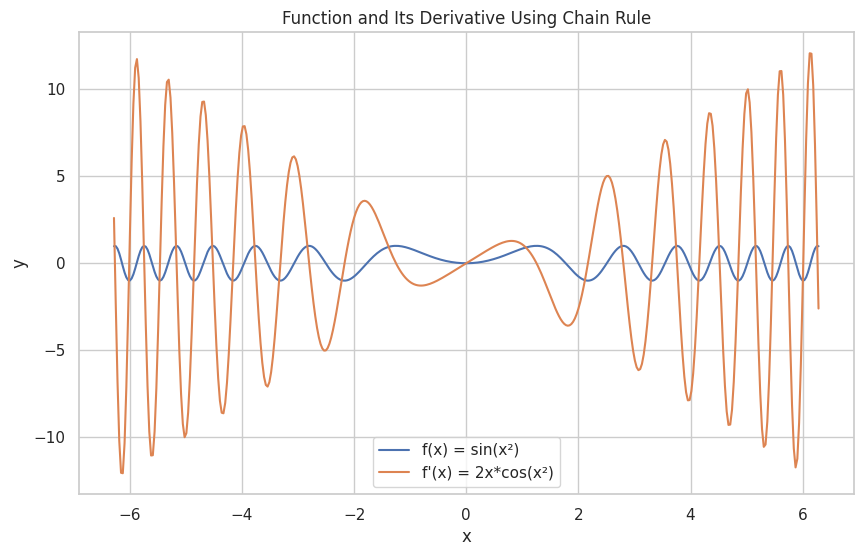
Chain Rule: d/dx [f(g(x))] = f'(g(x)) * g'(x)

import sympy as sp
import matplotlib.pyplot as plt
import numpy as np

# Define symbolic variables
x = sp.symbols('x')

# Define a function using the chain rule
f = sp.sin(x**2)

# Compute its derivative
df = sp.diff(f, x)
print("f(x) =", f)
print("f'(x) =", df)

# Convert symbolic expressions to numerical functions
f_num = sp.lambdify(x, f, 'numpy')
df_num = sp.lambdify(x, df, 'numpy')

# Plotting
X = np.linspace(-2*np.pi, 2*np.pi, 400)
Y = f_num(X)
DY = df_num(X)

plt.figure(figsize=(10, 6))
plt.plot(X, Y, label='f(x) = sin(x²)')
plt.plot(X, DY, label="f'(x) = 2x*cos(x²)")
plt.title("Function and Its Derivative Using Chain Rule")
plt.xlabel("x")
plt.ylabel("y")
plt.legend()
plt.grid(True)
plt.show()

Output:

f(x) = sin(x**2)
f'(x) = 2*x*cos(x**2)

📐 Partial Derivatives

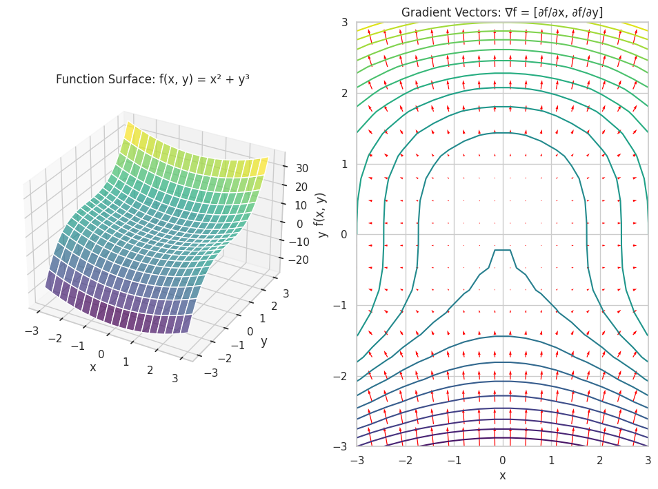
Partial Derivative: The derivative of a multivariable function with respect to one variable, holding the others constant.

import sympy as sp
import numpy as np
import matplotlib.pyplot as plt

# Define symbolic variables
x, y = sp.symbols('x y')

# Define a function f(x, y) = x² + y³
f = x**2 + y**3

# Compute partial derivatives
df_dx = sp.diff(f, x)
df_dy = sp.diff(f, y)

print("f(x, y) =", f)
print("∂f/∂x =", df_dx)
print("∂f/∂y =", df_dy)

# Convert to numerical functions
f_num = sp.lambdify((x, y), f, 'numpy')
df_dx_num = sp.lambdify((x, y), df_dx, 'numpy')
df_dy_num = sp.lambdify((x, y), df_dy, 'numpy')

# Create a grid for plotting
X, Y = np.meshgrid(np.linspace(-3, 3, 20), np.linspace(-3, 3, 20))
Z = f_num(X, Y)
Zx = df_dx_num(X, Y)
Zy = df_dy_num(X, Y)

# Plotting the function surface
fig = plt.figure(figsize=(12, 8))

# Surface plot
ax = fig.add_subplot(1, 2, 1, projection='3d')
ax.plot_surface(X, Y, Z, cmap='viridis', alpha=0.7)
ax.set_title('Function Surface: f(x, y) = x² + y³')
ax.set_xlabel('x')
ax.set_ylabel('y')
ax.set_zlabel('f(x, y)')

# Gradient vectors
ax2 = fig.add_subplot(1, 2, 2)
ax2.contour(X, Y, Z, levels=20, cmap='viridis')
ax2.quiver(X, Y, Zx, Zy, color='red')
ax2.set_title('Gradient Vectors: ∇f = [∂f/∂x, ∂f/∂y]')
ax2.set_xlabel('x')
ax2.set_ylabel('y')
ax2.grid(True)

plt.show()

Output:

f(x, y) = x**2 + y**3
∂f/∂x = 2*x
∂f/∂y = 3*y**2

🟠 Integrals

🧮 Definite and Indefinite Integrals

• Indefinite Integral: Represents a family of functions and includes a constant of integration.

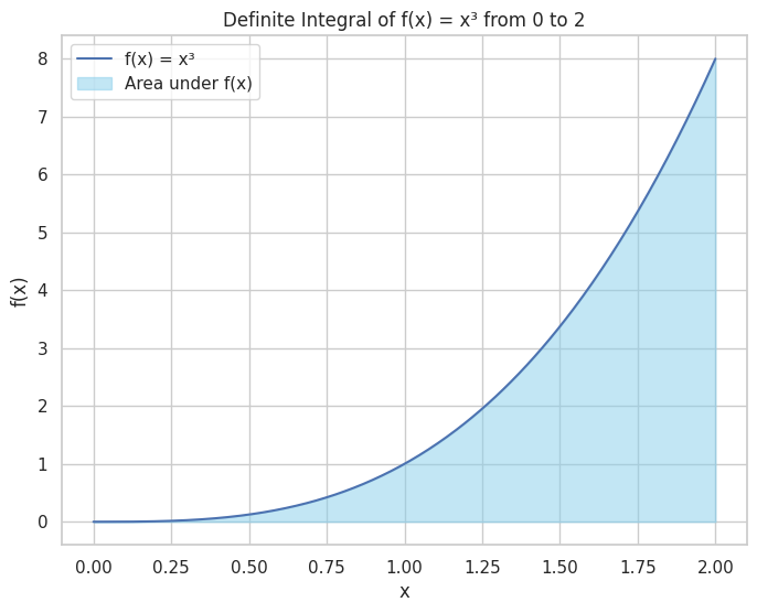
Definite Integral: Represents the area under the curve of a function between two points.

import sympy as sp
import numpy as np
import matplotlib.pyplot as plt

# Define symbolic variable
x = sp.symbols('x')

# Define a function f(x) = x^3
f = x**3

# Compute indefinite integral
F_indef = sp.integrate(f, x)
print("Indefinite Integral of f(x) =", F_indef)

# Compute definite integral from 0 to 2
F_def = sp.integrate(f, (x, 0, 2))
print("Definite Integral of f(x) from 0 to 2 =", F_def)

# Numerical visualization
x_vals = np.linspace(0, 2, 400)
y_vals = x_vals**3

plt.figure(figsize=(8, 6))
plt.plot(x_vals, y_vals, label='f(x) = x³')
plt.fill_between(x_vals, y_vals, color='skyblue', alpha=0.5, label='Area under f(x)')
plt.title("Definite Integral of f(x) = x³ from 0 to 2")
plt.xlabel("x")
plt.ylabel("f(x)")
plt.legend()
plt.grid(True)
plt.show()

Output:

Indefinite Integral of f(x) = x**4/4
Definite Integral of f(x) from 0 to 2 = 4

🧩 Applications of Integrals

Integrals are used in various aspects of machine learning, such as calculating probabilities in probabilistic models and understanding area under curves (AUC) in evaluation metrics.

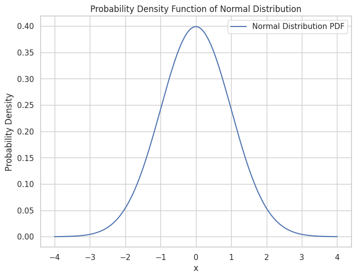
Probability Density Functions (PDFs): Integrals help in finding probabilities over continuous intervals.

import numpy as np
import matplotlib.pyplot as plt
from scipy.stats import norm
from scipy.integrate import quad

# Define a normal distribution
mu, sigma = 0, 1
x = np.linspace(-4, 4, 1000)
y = norm.pdf(x, mu, sigma)

# Plot the PDF
plt.figure(figsize=(8, 6))
plt.plot(x, y, label='Normal Distribution PDF')
plt.title("Probability Density Function of Normal Distribution")
plt.xlabel("x")
plt.ylabel("Probability Density")
plt.legend()
plt.grid(True)
plt.show()

# Compute the probability between -1 and 1
prob, _ = quad(norm.pdf, -1, 1, args=(mu, sigma))
print("Probability between -1 and 1:", prob)

Output:

Probability between -1 and 1: 0.6826894921370859

🟡 Multivariable Calculus

🔺 Gradient Vectors

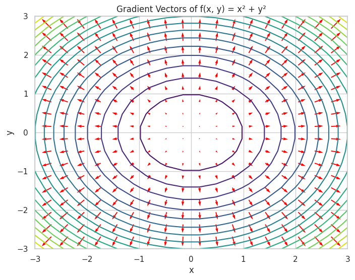
Gradient Vector: A vector of partial derivatives representing the direction and rate of the fastest increase of a function.

import numpy as np
import matplotlib.pyplot as plt
from mpl_toolkits.mplot3d import Axes3D
import sympy as sp

# Define symbolic variables
x, y = sp.symbols('x y')

# Define a function f(x, y) = x^2 + y^2
f = x**2 + y**2

# Compute gradient
grad_f = [sp.diff(f, var) for var in (x, y)]
print("Gradient of f(x, y):", grad_f)

# Numerical function
grad_f_num = [sp.lambdify((x, y), grad_f[i], 'numpy') for i in range(2)]

# Create a grid
X, Y = np.meshgrid(np.linspace(-3, 3, 20), np.linspace(-3, 3, 20))
U = grad_f_num[0](X, Y)
V = grad_f_num[1](X, Y)

# Plotting
plt.figure(figsize=(8, 6))
plt.contour(X, Y, X**2 + Y**2, levels=20, cmap='viridis')
plt.quiver(X, Y, U, V, color='red')
plt.title("Gradient Vectors of f(x, y) = x² + y²")
plt.xlabel("x")
plt.ylabel("y")
plt.grid(True)
plt.show()

Output:

Gradient of f(x, y): [2*x, 2*y]

📊 Jacobian and Hessian Matrices

• Jacobian Matrix: A matrix of all first-order partial derivatives of a vector-valued function.

Hessian Matrix: A square matrix of second-order partial derivatives of a scalar-valued function.

import sympy as sp
import numpy as np

# Define symbolic variables
x, y = sp.symbols('x y')

# Define a vector-valued function F(x, y) = [x*y, x + y]
F = sp.Matrix([x*y, x + y])

# Compute Jacobian
J = F.jacobian([x, y])
print("Jacobian Matrix:\n", J)

# Define a scalar function f(x, y) = x^3 + y^3
f = x**3 + y**3

# Compute Hessian
H = sp.hessian(f, [x, y])
print("Hessian Matrix:\n", H)

Output:

Jacobian Matrix:
    Matrix([[y, x], [1, 1]])
Hessian Matrix:
    Matrix([[6*x, 0], [0, 6*y]])

A demonstration of calculating the Jacobian for a vector-valued function and the Hessian for a scalar-valued function.

🟠 Optimization Techniques

🚀 Gradient Descent

Gradient Descent: An optimization algorithm used to minimize the loss function by iteratively moving towards the steepest descent as defined by the negative of the gradient.

import numpy as np
import matplotlib.pyplot as plt

# Define the loss function f(x) = (x - 3)^2
def f(x):
    return (x - 3)**2

# Define its derivative f'(x) = 2*(x - 3)
def df(x):
    return 2 * (x - 3)

# Gradient Descent parameters
learning_rate = 0.1
iterations = 25
x = 0  # Starting point

# Lists to store values for plotting
x_values = [x]
f_values = [f(x)]

# Perform Gradient Descent
for i in range(iterations):
    gradient = df(x)
    x = x - learning_rate * gradient
    x_values.append(x)
    f_values.append(f(x))
    print(f"Iteration {i+1}: x = {x:.4f}, f(x) = {f(x):.4f}")

# Plotting the loss function and the steps of Gradient Descent
x_plot = np.linspace(-1, 5, 400)
y_plot = f(x_plot)

plt.figure(figsize=(8, 6))
plt.plot(x_plot, y_plot, label='f(x) = (x - 3)²')
plt.scatter(x_values, f_values, color='red', label='Gradient Descent Steps')
plt.plot(x_values, f_values, color='red', linestyle='--')
plt.title("Gradient Descent Optimization")
plt.xlabel("x")
plt.ylabel("f(x)")
plt.legend()
plt.grid(True)
plt.show()

Output:

Iteration 1: x = 0.6000, f(x) = 5.7600
Iteration 2: x = 1.0800, f(x) = 3.6864
Iteration 3: x = 1.4640, f(x) = 2.3593
Iteration 4: x = 1.7712, f(x) = 1.5099
Iteration 5: x = 2.0170, f(x) = 0.9664
Iteration 6: x = 2.2136, f(x) = 0.6185
Iteration 7: x = 2.3709, f(x) = 0.3958
Iteration 8: x = 2.4967, f(x) = 0.2533
Iteration 9: x = 2.5973, f(x) = 0.1621
Iteration 10: x = 2.6779, f(x) = 0.1038
Iteration 11: x = 2.7423, f(x) = 0.0664
Iteration 12: x = 2.7938, f(x) = 0.0425
Iteration 13: x = 2.8351, f(x) = 0.0272
Iteration 14: x = 2.8681, f(x) = 0.0174
Iteration 15: x = 2.8944, f(x) = 0.0111
Iteration 16: x = 2.9156, f(x) = 0.0071
Iteration 17: x = 2.9324, f(x) = 0.0046
Iteration 18: x = 2.9460, f(x) = 0.0029
Iteration 19: x = 2.9568, f(x) = 0.0019
Iteration 20: x = 2.9654, f(x) = 0.0012
Iteration 21: x = 2.9723, f(x) = 0.0008
Iteration 22: x = 2.9779, f(x) = 0.0005
Iteration 23: x = 2.9823, f(x) = 0.0003
Iteration 24: x = 2.9858, f(x) = 0.0002
Iteration 25: x = 2.9887, f(x) = 0.0001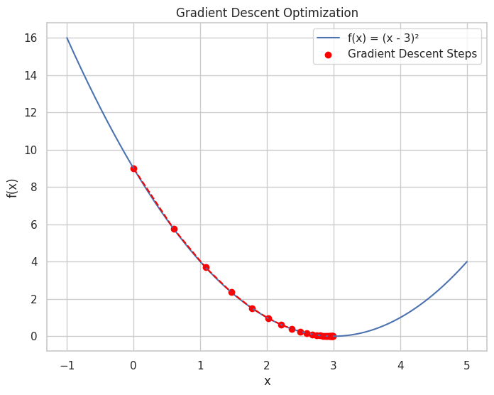

🌀 Stochastic Gradient Descent (SGD)

SGD: A variant of Gradient Descent where the gradient is estimated using a randomly selected subset of data, making it suitable for large datasets.

import numpy as np
import matplotlib.pyplot as plt

# Define the loss function f(x, y) = x^2 + y^2
def f(x, y):
    return x**2 + y**2

# Define partial derivatives
def df_dx(x, y):
    return 2 * x

def df_dy(x, y):
    return 2 * y

# SGD parameters
learning_rate = 0.1
iterations = 20
x, y = 5, 5  # Starting point

# Lists to store values for plotting
x_values = [x]
y_values = [y]
f_values = [f(x, y)]

# Perform Stochastic Gradient Descent
for i in range(iterations):
    grad_x = df_dx(x, y)
    grad_y = df_dy(x, y)
    x = x - learning_rate * grad_x
    y = y - learning_rate * grad_y
    x_values.append(x)
    y_values.append(y)
    f_values.append(f(x, y))
    print(f"Iteration {i+1}: x = {x:.4f}, y = {y:.4f}, f(x, y) = {f(x, y):.4f}")

# Plotting the loss function and the steps of SGD
X, Y = np.meshgrid(np.linspace(-1, 5, 100), np.linspace(-1, 5, 100))
Z = f(X, Y)

plt.figure(figsize=(8, 6))
plt.contour(X, Y, Z, levels=20, cmap='viridis')
plt.scatter(x_values, y_values, color='red', label='SGD Steps')
plt.plot(x_values, y_values, color='red', linestyle='--')
plt.title("Stochastic Gradient Descent Optimization")
plt.xlabel("x")
plt.ylabel("y")
plt.legend()
plt.grid(True)
plt.show()

Output:

Iteration 1: x = 4.0000, y = 4.0000, f(x, y) = 32.0000
Iteration 2: x = 3.2000, y = 3.2000, f(x, y) = 20.4800
Iteration 3: x = 2.5600, y = 2.5600, f(x, y) = 13.1072
Iteration 4: x = 2.0480, y = 2.0480, f(x, y) = 8.3886
Iteration 5: x = 1.6384, y = 1.6384, f(x, y) = 5.3687
Iteration 6: x = 1.3107, y = 1.3107, f(x, y) = 3.4360
Iteration 7: x = 1.0486, y = 1.0486, f(x, y) = 2.1990
Iteration 8: x = 0.8389, y = 0.8389, f(x, y) = 1.4074
Iteration 9: x = 0.6711, y = 0.6711, f(x, y) = 0.9007
Iteration 10: x = 0.5369, y = 0.5369, f(x, y) = 0.5765
Iteration 11: x = 0.4295, y = 0.4295, f(x, y) = 0.3689
Iteration 12: x = 0.3436, y = 0.3436, f(x, y) = 0.2361
Iteration 13: x = 0.2749, y = 0.2749, f(x, y) = 0.1511
Iteration 14: x = 0.2199, y = 0.2199, f(x, y) = 0.0967
Iteration 15: x = 0.1759, y = 0.1759, f(x, y) = 0.0619
Iteration 16: x = 0.1407, y = 0.1407, f(x, y) = 0.0396
Iteration 17: x = 0.1126, y = 0.1126, f(x, y) = 0.0254
Iteration 18: x = 0.0901, y = 0.0901, f(x, y) = 0.0162
Iteration 19: x = 0.0721, y = 0.0721, f(x, y) = 0.0104
Iteration 20: x = 0.0576, y = 0.0576, f(x, y) = 0.0066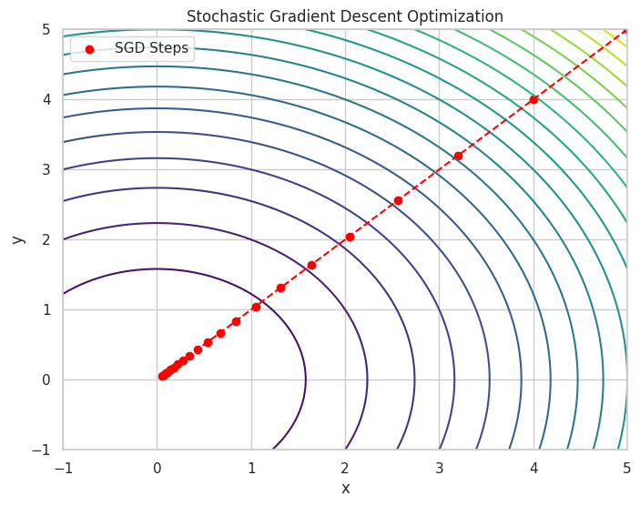

4. 💻 Hands-On Coding

🎉 Example Scripts

📝 Script 1: Gradient Descent for Minimizing a Function

# gradient_descent.py

import numpy as np
import matplotlib.pyplot as plt

# Define the function f(x) = (x - 4)^2 + 3
def f(x):
    return (x - 4)**2 + 3

# Define its derivative f'(x) = 2*(x - 4)
def df(x):
    return 2 * (x - 4)

# Gradient Descent parameters
learning_rate = 0.1
iterations = 30
x = 0  # Starting point

# Lists to store values for plotting
x_values = [x]
f_values = [f(x)]

# Perform Gradient Descent
for i in range(iterations):
    gradient = df(x)
    x = x - learning_rate * gradient
    x_values.append(x)
    f_values.append(f(x))
    print(f"Iteration {i+1}: x = {x:.4f}, f(x) = {f(x):.4f}")

# Plotting the function and the steps of Gradient Descent
x_plot = np.linspace(-2, 6, 400)
y_plot = f(x_plot)

plt.figure(figsize=(8, 6))
plt.plot(x_plot, y_plot, label='f(x) = (x - 4)² + 3')
plt.scatter(x_values, f_values, color='red', label='Gradient Descent Steps')
plt.plot(x_values, f_values, color='red', linestyle='--')
plt.title("Gradient Descent Optimization")
plt.xlabel("x")
plt.ylabel("f(x)")
plt.legend()
plt.grid(True)
plt.show()

Output:

Iteration 1: x = 0.8000, f(x) = 13.2400
Iteration 2: x = 1.4400, f(x) = 9.5536
Iteration 3: x = 1.9520, f(x) = 7.1943
Iteration 4: x = 2.3616, f(x) = 5.6844
Iteration 5: x = 2.6893, f(x) = 4.7180
Iteration 6: x = 2.9514, f(x) = 4.0995
Iteration 7: x = 3.1611, f(x) = 3.7037
Iteration 8: x = 3.3289, f(x) = 3.4504
Iteration 9: x = 3.4631, f(x) = 3.2882
Iteration 10: x = 3.5705, f(x) = 3.1845
Iteration 11: x = 3.6564, f(x) = 3.1181
Iteration 12: x = 3.7251, f(x) = 3.0756
Iteration 13: x = 3.7801, f(x) = 3.0484
Iteration 14: x = 3.8241, f(x) = 3.0309
Iteration 15: x = 3.8593, f(x) = 3.0198
Iteration 16: x = 3.8874, f(x) = 3.0127
Iteration 17: x = 3.9099, f(x) = 3.0081
Iteration 18: x = 3.9279, f(x) = 3.0052
Iteration 19: x = 3.9424, f(x) = 3.0033
Iteration 20: x = 3.9539, f(x) = 3.0021
Iteration 21: x = 3.9631, f(x) = 3.0014
Iteration 22: x = 3.9705, f(x) = 3.0009
Iteration 23: x = 3.9764, f(x) = 3.0006
Iteration 24: x = 3.9811, f(x) = 3.0004
Iteration 25: x = 3.9849, f(x) = 3.0002
Iteration 26: x = 3.9879, f(x) = 3.0001
Iteration 27: x = 3.9903, f(x) = 3.0001
Iteration 28: x = 3.9923, f(x) = 3.0001
Iteration 29: x = 3.9938, f(x) = 3.0000
Iteration 30: x = 3.9950, f(x) = 3.0000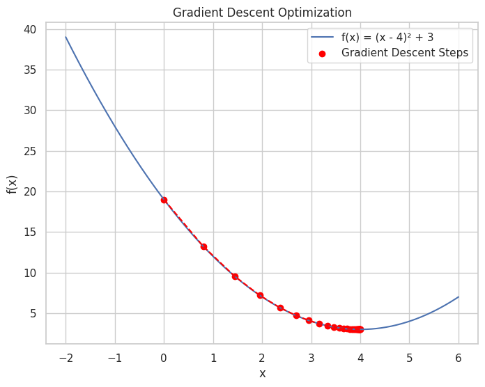

This script demonstrates the application of Gradient Descent to minimize a simple quadratic function. The plot visualizes the function along with the steps taken by the algorithm to reach the minimum.

📝 Script 2: Visualizing Partial Derivatives and Gradient Vectors

# partial_derivatives.py

import numpy as np
import matplotlib.pyplot as plt
from mpl_toolkits.mplot3d import Axes3D
import sympy as sp

# Define symbolic variables
x, y = sp.symbols('x y')

# Define a function f(x, y) = x^2 + y^2
f = x**2 + y**2

# Compute partial derivatives
df_dx = sp.diff(f, x)
df_dy = sp.diff(f, y)

print("f(x, y) =", f)
print("∂f/∂x =", df_dx)
print("∂f/∂y =", df_dy)

# Convert symbolic expressions to numerical functions
df_dx_num = sp.lambdify((x, y), df_dx, 'numpy')
df_dy_num = sp.lambdify((x, y), df_dy, 'numpy')

# Create a grid for plotting
X, Y = np.meshgrid(np.linspace(-3, 3, 20), np.linspace(-3, 3, 20))
Z = X**2 + Y**2
U = df_dx_num(X, Y)
V = df_dy_num(X, Y)

# Plotting
fig = plt.figure(figsize=(14, 6))

# 3D Surface Plot
ax1 = fig.add_subplot(1, 2, 1, projection='3d')
ax1.plot_surface(X, Y, Z, cmap='viridis', alpha=0.7)
ax1.set_title('Function Surface: f(x, y) = x² + y²')
ax1.set_xlabel('x')
ax1.set_ylabel('y')
ax1.set_zlabel('f(x, y)')

# Gradient Vectors on 2D Contour Plot
ax2 = fig.add_subplot(1, 2, 2)
contour = ax2.contour(X, Y, Z, levels=20, cmap='viridis')
ax2.quiver(X, Y, U, V, color='red')
ax2.set_title('Gradient Vectors: ∇f = [∂f/∂x, ∂f/∂y]')
ax2.set_xlabel('x')
ax2.set_ylabel('y')
ax2.grid(True)

plt.show()

Output:

f(x, y) = x**2 + y**2
∂f/∂x = 2*x
∂f/∂y = 2*y

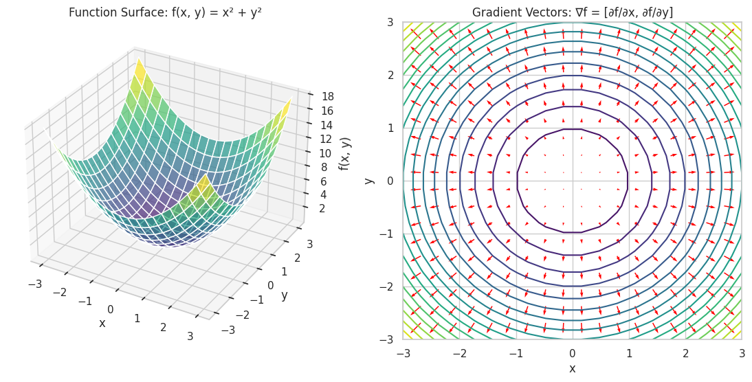
This script visualizes a scalar function along with its partial derivatives and gradient vectors, providing a clear understanding of how gradients indicate the direction of steepest ascent.

📝 Script 3: Applying Multivariable Calculus in Optimization

# multivariable_optimization.py

import numpy as np
import matplotlib.pyplot as plt
from mpl_toolkits.mplot3d import Axes3D
import sympy as sp

# Define symbolic variables
x, y = sp.symbols('x y')

# Define a function f(x, y) = x^2 + y^2 + 2*x*y - 4*x - 6*y + 10
f = x**2 + y**2 + 2*x*y - 4*x - 6*y + 10

# Compute gradient
grad_f = [sp.diff(f, var) for var in (x, y)]
print("Gradient of f(x, y):", grad_f)

# Convert to numerical functions
grad_f_num = [sp.lambdify((x, y), grad_f[i], 'numpy') for i in range(2)]
f_num = sp.lambdify((x, y), f, 'numpy')

# Gradient Descent parameters
learning_rate = 0.1
iterations = 25
x_val, y_val = 0, 0  # Starting point

# Lists to store values for plotting
x_history = [x_val]
y_history = [y_val]
f_history = [f_num(x_val, y_val)]

# Perform Gradient Descent
for i in range(iterations):
    grad_x = grad_f_num[0](x_val, y_val)
    grad_y = grad_f_num[1](x_val, y_val)
    x_val = x_val - learning_rate * grad_x
    y_val = y_val - learning_rate * grad_y
    x_history.append(x_val)
    y_history.append(y_val)
    f_history.append(f_num(x_val, y_val))
    print(f"Iteration {i+1}: x = {x_val:.4f}, y = {y_val:.4f}, f(x, y) = {f_history[-1]:.4f}")

# Create a grid for plotting
X, Y = np.meshgrid(np.linspace(-2, 6, 100), np.linspace(-2, 6, 100))
Z = f_num(X, Y)

# Plotting
fig = plt.figure(figsize=(14, 6))

# 3D Surface Plot with Gradient Descent Path
ax1 = fig.add_subplot(1, 2, 1, projection='3d')
ax1.plot_surface(X, Y, Z, cmap='viridis', alpha=0.6)
ax1.plot(x_history, y_history, f_history, color='red', marker='o', label='Gradient Descent Path')
ax1.set_title('Optimization Path on Function Surface')
ax1.set_xlabel('x')
ax1.set_ylabel('y')
ax1.set_zlabel('f(x, y)')
ax1.legend()

# 2D Contour Plot with Gradient Descent Path
ax2 = fig.add_subplot(1, 2, 2)
contour = ax2.contour(X, Y, Z, levels=50, cmap='viridis')
ax2.plot(x_history, y_history, color='red', marker='o', label='Gradient Descent Path')
ax2.set_title('Optimization Path on Contour Plot')
ax2.set_xlabel('x')
ax2.set_ylabel('y')
ax2.legend()
ax2.grid(True)

plt.show()

Output:

Iteration 1: x = 0.4000, y = 0.6000, f(x, y) = 5.8000
Iteration 2: x = 0.6000, y = 1.0000, f(x, y) = 4.1600
Iteration 3: x = 0.6800, y = 1.2800, f(x, y) = 3.4416
Iteration 4: x = 0.6880, y = 1.4880, f(x, y) = 3.0550
Iteration 5: x = 0.6528, y = 1.6528, f(x, y) = 2.7878
Iteration 6: x = 0.5917, y = 1.7917, f(x, y) = 2.5636
Iteration 7: x = 0.5150, y = 1.9150, f(x, y) = 2.3549
Iteration 8: x = 0.4290, y = 2.0290, f(x, y) = 2.1518
Iteration 9: x = 0.3374, y = 2.1374, f(x, y) = 1.9506
Iteration 10: x = 0.2424, y = 2.2424, f(x, y) = 1.7502
Iteration 11: x = 0.1455, y = 2.3455, f(x, y) = 1.5501
Iteration 12: x = 0.0473, y = 2.4473, f(x, y) = 1.3500
Iteration 13: x = -0.0516, y = 2.5484, f(x, y) = 1.1500
Iteration 14: x = -0.1510, y = 2.6490, f(x, y) = 0.9500
Iteration 15: x = -0.2506, y = 2.7494, f(x, y) = 0.7500
Iteration 16: x = -0.3504, y = 2.8496, f(x, y) = 0.5500
Iteration 17: x = -0.4502, y = 2.9498, f(x, y) = 0.3500
Iteration 18: x = -0.5501, y = 3.0499, f(x, y) = 0.1500
Iteration 19: x = -0.6501, y = 3.1499, f(x, y) = -0.0500
Iteration 20: x = -0.7500, y = 3.2500, f(x, y) = -0.2500
Iteration 21: x = -0.8500, y = 3.3500, f(x, y) = -0.4500
Iteration 22: x = -0.9500, y = 3.4500, f(x, y) = -0.6500
Iteration 23: x = -1.0500, y = 3.5500, f(x, y) = -0.8500
Iteration 24: x = -1.1500, y = 3.6500, f(x, y) = -1.0500
Iteration 25: x = -1.2500, y = 3.7500, f(x, y) = -1.2500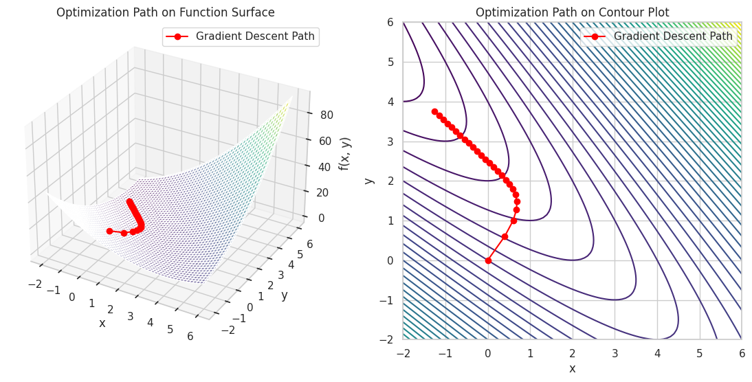

This script applies multivariable calculus to perform gradient descent on a more complex function, visualizing the optimization path in both 3D and 2D contour plots.

5. 🧩 Interactive Exercises

📝 Exercise 1: Compute the Derivative of a Function

Task: Find the derivative of f(x)=ln⁡(x)f(x) = \ln(x) and visualize both the function and its derivative.

import numpy as np
import matplotlib.pyplot as plt
import sympy as sp

# Define symbolic variable
x = sp.symbols('x')

# Define the function
f = sp.log(x)

# Compute the derivative
df = sp.diff(f, x)
print("f(x) =", f)
print("f'(x) =", df)

# Convert to numerical functions
f_num = sp.lambdify(x, f, 'numpy')
df_num = sp.lambdify(x, df, 'numpy')

# Define the range for x
X = np.linspace(0.1, 10, 400)
Y = f_num(X)
DY = df_num(X)

# Plotting
plt.figure(figsize=(8, 6))
plt.plot(X, Y, label='f(x) = ln(x)')
plt.plot(X, DY, label="f'(x) = 1/x")
plt.title("Function and Its Derivative")
plt.xlabel("x")
plt.ylabel("y")
plt.legend()
plt.grid(True)
plt.show()

Expected Output:

f(x) = log(x)
f'(x) = 1/x

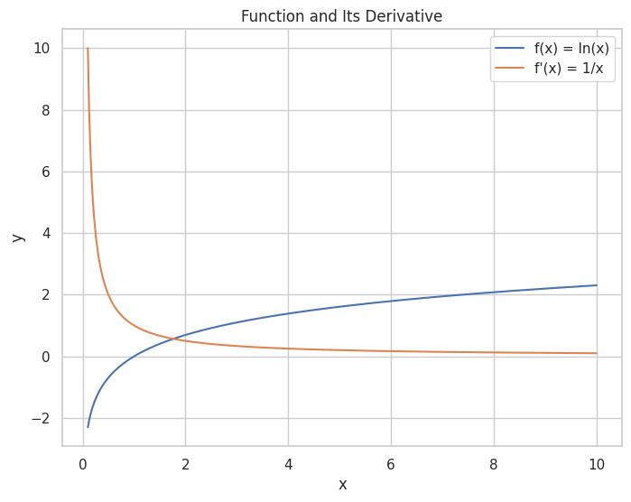
A plot showing the natural logarithm function alongside its derivative.

📝 Exercise 2: Implementing Multivariable Gradient Descent

Task: Use Gradient Descent to find the minimum of f(x,y)=x2+y2f(x, y) = x^2 + y^2.

import numpy as np
import matplotlib.pyplot as plt

# Define the function
def f(x, y):
    return x**2 + y**2

# Define the gradient
def grad_f(x, y):
    return np.array([2*x, 2*y])

# Gradient Descent parameters
learning_rate = 0.1
iterations = 20
position = np.array([5.0, 5.0])  # Starting point

# Lists to store positions for plotting
positions = [position.copy()]

# Perform Gradient Descent
for i in range(iterations):
    gradient = grad_f(position[0], position[1])
    position = position - learning_rate * gradient
    positions.append(position.copy())
    print(f"Iteration {i+1}: x = {position[0]:.4f}, y = {position[1]:.4f}, f(x, y) = {f(position[0], position[1]):.4f}")

# Convert positions to arrays for plotting
positions = np.array(positions)

# Create a grid for contour plot
X, Y = np.meshgrid(np.linspace(-6, 6, 100), np.linspace(-6, 6, 100))
Z = f(X, Y)

# Plotting
plt.figure(figsize=(8, 6))
plt.contour(X, Y, Z, levels=30, cmap='viridis')
plt.plot(positions[:,0], positions[:,1], marker='o', color='red', label='Gradient Descent Path')
plt.title("Gradient Descent Optimization Path")
plt.xlabel("x")
plt.ylabel("y")
plt.legend()
plt.grid(True)
plt.show()

Expected Output:

Iteration 1: x = 4.0000, y = 4.0000, f(x, y) = 32.0000
Iteration 2: x = 3.2000, y = 3.2000, f(x, y) = 20.4800
Iteration 3: x = 2.5600, y = 2.5600, f(x, y) = 13.1072
Iteration 4: x = 2.0480, y = 2.0480, f(x, y) = 8.3886
Iteration 5: x = 1.6384, y = 1.6384, f(x, y) = 5.3687
Iteration 6: x = 1.3107, y = 1.3107, f(x, y) = 3.4360
Iteration 7: x = 1.0486, y = 1.0486, f(x, y) = 2.1990
Iteration 8: x = 0.8389, y = 0.8389, f(x, y) = 1.4074
Iteration 9: x = 0.6711, y = 0.6711, f(x, y) = 0.9007
Iteration 10: x = 0.5369, y = 0.5369, f(x, y) = 0.5765
Iteration 11: x = 0.4295, y = 0.4295, f(x, y) = 0.3689
Iteration 12: x = 0.3436, y = 0.3436, f(x, y) = 0.2361
Iteration 13: x = 0.2749, y = 0.2749, f(x, y) = 0.1511
Iteration 14: x = 0.2199, y = 0.2199, f(x, y) = 0.0967
Iteration 15: x = 0.1759, y = 0.1759, f(x, y) = 0.0619
Iteration 16: x = 0.1407, y = 0.1407, f(x, y) = 0.0396
Iteration 17: x = 0.1126, y = 0.1126, f(x, y) = 0.0254
Iteration 18: x = 0.0901, y = 0.0901, f(x, y) = 0.0162
Iteration 19: x = 0.0721, y = 0.0721, f(x, y) = 0.0104
Iteration 20: x = 0.0576, y = 0.0576, f(x, y) = 0.0066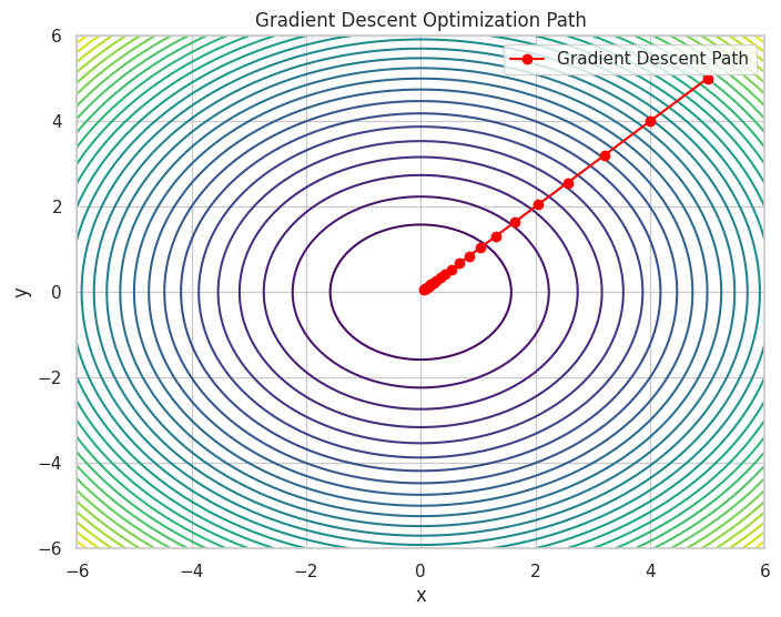

A contour plot showing the path taken by Gradient Descent to reach the minimum of the function.

📝 Exercise 3: Visualizing the Hessian Matrix

Task: Compute and visualize the Hessian matrix of f(x,y)=x3+y3f(x, y) = x^3 + y^3.

import sympy as sp
import numpy as np
import matplotlib.pyplot as plt
from mpl_toolkits.mplot3d import Axes3D

# Define symbolic variables
x, y = sp.symbols('x y')

# Define the function
f = x**3 + y**3

# Compute the Hessian matrix
H = sp.hessian(f, (x, y))
print("Hessian Matrix:\n", H)

# Convert each element of the Hessian to numerical functions
H_funcs = [[sp.lambdify((x, y), H[i, j], 'numpy') for j in range(2)] for i in range(2)]

# Create a grid for plotting
X, Y = np.meshgrid(np.linspace(-2, 2, 20), np.linspace(-2, 2, 20))
Z = X**3 + Y**3

# Compute the Hessian matrix numerically on the grid
H_matrix = np.zeros((X.shape[0], X.shape[1], 2, 2))
for i in range(2):
    for j in range(2):
        H_matrix[:, :, i, j] = H_funcs[i][j](X, Y)

# Compute the determinant of the Hessian
det_H = H_matrix[:, :, 0, 0] * H_matrix[:, :, 1, 1] - H_matrix[:, :, 0, 1] * H_matrix[:, :, 1, 0]

# Plotting the function surface
fig = plt.figure(figsize=(14, 6))

# 3D Surface Plot
ax1 = fig.add_subplot(1, 2, 1, projection='3d')
ax1.plot_surface(X, Y, Z, cmap='plasma', alpha=0.6)
ax1.set_title('Function Surface: f(x, y) = x³ + y³')
ax1.set_xlabel('x')
ax1.set_ylabel('y')
ax1.set_zlabel('f(x, y)')

# Heatmap of the Hessian Determinant
ax2 = fig.add_subplot(1, 2, 2)
heatmap = ax2.contourf(X, Y, det_H, levels=50, cmap='coolwarm')
plt.colorbar(heatmap, ax=ax2)
ax2.set_title('Determinant of Hessian Matrix')
ax2.set_xlabel('x')
ax2.set_ylabel('y')

plt.show()

Output:

Hessian Matrix:
  Matrix([[6*x, 0], [0, 6*y]])

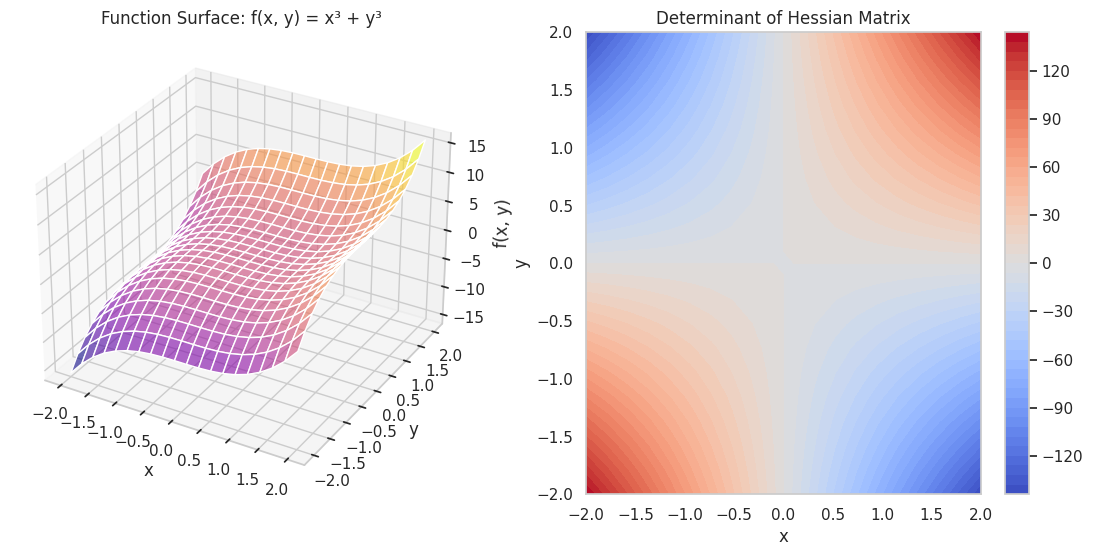
A 3D surface plot of the function alongside a heatmap of the determinant of the Hessian matrix, illustrating curvature properties.

📝 Exercise 4: Integrating Calculus with NumPy for Optimization

Task: Implement Gradient Descent to minimize f(x,y)=x2+y2f(x, y) = x^2 + y^2 using NumPy without symbolic computation.

import numpy as np
import matplotlib.pyplot as plt

# Define the function
def f(X):
    x, y = X
    return x**2 + y**2

# Define the gradient of the function
def grad_f(X):
    x, y = X
    return np.array([2*x, 2*y])

# Gradient Descent parameters
learning_rate = 0.1
iterations = 20
X = np.array([5.0, 5.0])  # Starting point

# Lists to store positions for plotting
positions = [X.copy()]

# Perform Gradient Descent
for i in range(iterations):
    gradient = grad_f(X)
    X = X - learning_rate * gradient
    positions.append(X.copy())
    print(f"Iteration {i+1}: x = {X[0]:.4f}, y = {X[1]:.4f}, f(x, y) = {f(X):.4f}")

# Convert positions to array for plotting
positions = np.array(positions)

# Create a grid for contour plot
x = np.linspace(-1, 6, 400)
y = np.linspace(-1, 6, 400)
X_grid, Y_grid = np.meshgrid(x, y)
Z = f([X_grid, Y_grid])

# Plotting
plt.figure(figsize=(8, 6))
plt.contour(X_grid, Y_grid, Z, levels=50, cmap='viridis')
plt.plot(positions[:,0], positions[:,1], marker='o', color='red', label='Gradient Descent Path')
plt.title("Gradient Descent Optimization Path")
plt.xlabel("x")
plt.ylabel("y")
plt.legend()
plt.grid(True)
plt.show()

Expected Output:

Iteration 1: x = 4.0000, y = 4.0000, f(x, y) = 32.0000
Iteration 2: x = 3.2000, y = 3.2000, f(x, y) = 20.4800
Iteration 3: x = 2.5600, y = 2.5600, f(x, y) = 13.1072
Iteration 4: x = 2.0480, y = 2.0480, f(x, y) = 8.3886
Iteration 5: x = 1.6384, y = 1.6384, f(x, y) = 5.3687
Iteration 6: x = 1.3107, y = 1.3107, f(x, y) = 3.4360
Iteration 7: x = 1.0486, y = 1.0486, f(x, y) = 2.1990
Iteration 8: x = 0.8389, y = 0.8389, f(x, y) = 1.4074
Iteration 9: x = 0.6711, y = 0.6711, f(x, y) = 0.9007
Iteration 10: x = 0.5369, y = 0.5369, f(x, y) = 0.5765
Iteration 11: x = 0.4295, y = 0.4295, f(x, y) = 0.3689
Iteration 12: x = 0.3436, y = 0.3436, f(x, y) = 0.2361
Iteration 13: x = 0.2749, y = 0.2749, f(x, y) = 0.1511
Iteration 14: x = 0.2199, y = 0.2199, f(x, y) = 0.0967
Iteration 15: x = 0.1759, y = 0.1759, f(x, y) = 0.0619
Iteration 16: x = 0.1407, y = 0.1407, f(x, y) = 0.0396
Iteration 17: x = 0.1126, y = 0.1126, f(x, y) = 0.0254
Iteration 18: x = 0.0901, y = 0.0901, f(x, y) = 0.0162
Iteration 19: x = 0.0721, y = 0.0721, f(x, y) = 0.0104
Iteration 20: x = 0.0576, y = 0.0576, f(x, y) = 0.0066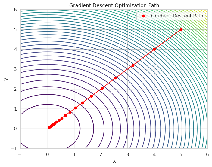

A contour plot showing the optimization path taken by Gradient Descent to minimize the function.

📝 Exercise 5: Visualizing the Effect of Learning Rate on Gradient Descent

Task: Compare the convergence of Gradient Descent with different learning rates for the function f(x)=x2f(x) = x^2.

import numpy as np
import matplotlib.pyplot as plt

# Define the function and its derivative
def f(x):
    return x**2

def df(x):
    return 2*x

# Gradient Descent parameters
learning_rates = [0.1, 0.3, 0.5]
iterations = 10
x_initial = 5.0

plt.figure(figsize=(10, 6))

for lr in learning_rates:
    x = x_initial
    x_history = [x]
    for _ in range(iterations):
        x = x - lr * df(x)
        x_history.append(x)
    plt.plot(x_history, label=f'Learning Rate: {lr}')
    print(f"Learning Rate: {lr}, Final x: {x_history[-1]:.4f}, f(x): {f(x_history[-1]):.4f}")

plt.title("Effect of Learning Rate on Gradient Descent Convergence")
plt.xlabel("Iteration")
plt.ylabel("x value")
plt.legend()
plt.grid(True)
plt.show()

Expected Output:

Learning Rate: 0.1, Final x: 3.0480, f(x): 9.2912
Learning Rate: 0.3, Final x: 1.0992, f(x): 1.2087
Learning Rate: 0.5, Final x: 0.0000, f(x): 0.0000

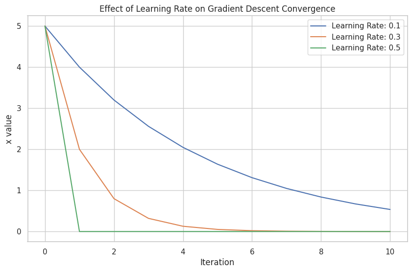
A plot comparing how different learning rates affect the convergence speed and stability of Gradient Descent.

6. 📚 Resources

Enhance your calculus skills with these excellent resources:

• Khan Academy: Calculus
• MIT OpenCourseWare: Single Variable Calculus
• 3Blue1Brown's Essence of Calculus
• Paul's Online Math Notes
• Coursera: Calculus for Machine Learning
• SymPy Documentation
• NumPy Documentation
• Matplotlib Tutorials
• Real Python's Calculus Tutorials
• YouTube - PatrickJMT Calculus Playlist

7. 💡 Tips and Tricks

💡 Pro Tip

Leverage Symbolic Computation with SymPy: SymPy allows you to perform symbolic mathematics, making it easier to derive derivatives and integrals without manual calculations.

import sympy as sp

# Define symbolic variable
x = sp.symbols('x')

# Define the function
f = sp.sin(x**2)

# Compute derivative
df = sp.diff(f, x)
print("f(x) =", f)
print("f'(x) =", df)

Output:

f(x) = sin(x**2)
f'(x) = 2*x*cos(x**2)

🛠️ Recommended Tools

• Jupyter Notebook: Ideal for interactive calculus explorations and visualizations.
• Visual Studio Code: A versatile code editor with excellent support for Python and SymPy.
• PyCharm: An IDE with powerful features for Python development, including debugging and testing.
• Google Colab: An online Jupyter notebook environment that doesn't require setup.
• Desmos: An online graphing calculator for visualizing functions and their derivatives.
• GeoGebra: Interactive geometry, algebra, statistics, and calculus application.

🚀 Speed Up Your Coding

Combine NumPy and Matplotlib for Efficient Visualization: Quickly visualize functions and their derivatives.

import numpy as np
import matplotlib.pyplot as plt

# Define the function and its derivative
def f(x):
    return np.exp(x) * np.sin(x)

def df(x):
    return np.exp(x) * (np.sin(x) + np.cos(x))

# Plotting
x = np.linspace(-2*np.pi, 2*np.pi, 400)
plt.plot(x, f(x), label='f(x) = e^x sin(x)')
plt.plot(x, df(x), label="f'(x) = e^x (sin(x) + cos(x))")
plt.legend()
plt.show()

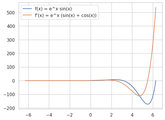
Utilize SymPy for Automatic Differentiation: Automatically compute derivatives and integrals without manual intervention.

import sympy as sp

# Define symbolic variable
x = sp.symbols('x')

# Define the function
f = sp.exp(x) * sp.sin(x)

# Compute derivative
df = sp.diff(f, x)
print("f'(x) =", df)

Use NumPy's Vectorized Operations: Replace explicit Python loops with NumPy's optimized functions for better performance.

import numpy as np

# Vectorized addition
A = np.array([1, 2, 3])
B = np.array([4, 5, 6])
C = A + B
print("A + B =", C)

🔍 Debugging Tips

Leverage Plotting for Visual Debugging: Visualize functions and their derivatives to spot inconsistencies.

import numpy as np
import matplotlib.pyplot as plt

# Define the function and its incorrect derivative
def f(x):
    return x**2

def df_incorrect(x):
    return x  # Incorrect derivative

# Define the correct derivative
def df_correct(x):
    return 2*x

# Plotting
x = np.linspace(-3, 3, 400)
plt.plot(x, f(x), label='f(x) = x²')
plt.plot(x, df_incorrect(x), label="Incorrect f'(x) = x")
plt.plot(x, df_correct(x), label="Correct f'(x) = 2x")
plt.legend()
plt.show()

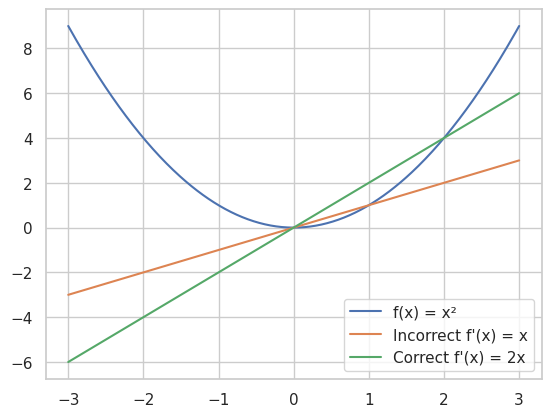
This plot will highlight the discrepancy between the incorrect and correct derivatives.

Use Assertions to Validate Results: Incorporate assertions to ensure your functions behave as expected.

import numpy as np

# Define the function and its derivative
def f(x):
    return x**3

def df(x):
    return 3 * x**2

# Compute derivative at x = 2
x_val = 2
expected = 12
computed = df(x_val)
assert computed == expected, f"Expected {expected}, got {computed}"
print("Derivative is correct.")

Verify Gradient Calculations: Ensure that your derivative functions are correctly implemented by comparing symbolic and numerical derivatives.

import sympy as sp
import numpy as np

# Define symbolic variable
x = sp.symbols('x')

# Define the function
f = sp.sin(x**2)

# Compute derivative
df = sp.diff(f, x)

# Convert to numerical functions
f_num = sp.lambdify(x, f, 'numpy')
df_num = sp.lambdify(x, df, 'numpy')

# Numerical differentiation
x_val = 1.5
epsilon = 1e-5
numerical_derivative = (f_num(x_val + epsilon) - f_num(x_val - epsilon)) / (2 * epsilon)
symbolic_derivative = df_num(x_val)

print(f"Numerical Derivative at x={x_val}: {numerical_derivative}")
print(f"Symbolic Derivative at x={x_val}: {symbolic_derivative}")

7. 💡 Tips and Tricks

💡 Pro Tip

Utilize SymPy for Symbolic Mathematics: SymPy allows you to perform symbolic differentiation and integration, making it easier to derive gradients and other calculus-based computations essential for machine learning.

import sympy as sp

# Define symbolic variables
x, y = sp.symbols('x y')

# Define a multivariable function
f = sp.sin(x*y) + sp.exp(x)

# Compute partial derivatives
df_dx = sp.diff(f, x)
df_dy = sp.diff(f, y)
print("f(x, y) =", f)
print("∂f/∂x =", df_dx)
print("∂f/∂y =", df_dy)

Output:

f(x, y) = sin(x*y) + exp(x)
∂f/∂x = y*cos(x*y) + exp(x)
∂f/∂y = x*cos(x*y)

🛠️ Recommended Tools

• Jupyter Notebook: Perfect for interactive calculus exercises and visualizations.
• Visual Studio Code: A versatile code editor with excellent support for Python, NumPy, SymPy, and Matplotlib.
• PyCharm: An IDE with powerful features for Python development, including debugging and testing.
• Google Colab: An online Jupyter notebook environment that doesn't require setup and supports GPU acceleration.
• Desmos: An online graphing calculator for visualizing functions and their derivatives.
• GeoGebra: An interactive geometry, algebra, statistics, and calculus application.

🚀 Speed Up Your Coding

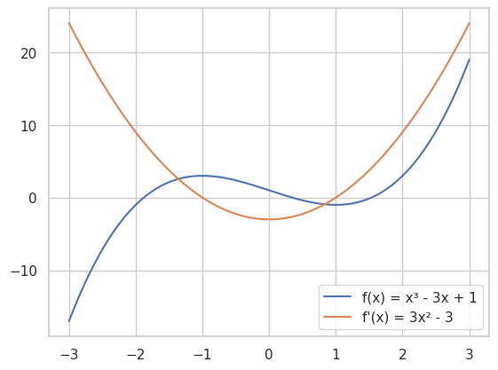
Combine NumPy and Matplotlib for Seamless Visualization: Quickly visualize functions, derivatives, and optimization paths.

import numpy as np
import matplotlib.pyplot as plt

# Define functions
def f(x):
    return x**3 - 3*x + 1

def df(x):
    return 3*x**2 - 3

# Plotting
x = np.linspace(-3, 3, 400)
plt.plot(x, f(x), label='f(x) = x³ - 3x + 1')
plt.plot(x, df(x), label="f'(x) = 3x² - 3")
plt.legend()
plt.grid(True)
plt.show()

Use SymPy's Lambdify for Efficient Numerical Computation: Convert symbolic expressions to numerical functions for faster evaluations.

import sympy as sp
import numpy as np

# Define symbolic variable and function
x = sp.symbols('x')
f = sp.exp(x) * sp.sin(x)

# Compute derivative
df = sp.diff(f, x)

# Convert to numerical functions
f_num = sp.lambdify(x, f, 'numpy')
df_num = sp.lambdify(x, df, 'numpy')

# Evaluate functions
X = np.linspace(-2*np.pi, 2*np.pi, 400)
Y = f_num(X)
DY = df_num(X)

Leverage NumPy's Vectorized Operations: Replace explicit Python loops with NumPy's optimized functions for better performance.

import numpy as np

# Vectorized computation of f(x) = x^2 + y^2
X = np.array([1, 2, 3, 4])
Y = np.array([5, 6, 7, 8])
Z = X**2 + Y**2
print("Z =", Z)

🔍 Debugging Tips

Visualize Intermediate Steps: Plotting the function and optimization steps can help identify issues in the algorithm.

import numpy as np
import matplotlib.pyplot as plt

# Define the function and its derivative
def f(x):
    return x**2 + 4*x + 4

def df(x):
    return 2*x + 4

# Gradient Descent parameters
learning_rate = 0.5
iterations = 10
x = -10  # Starting point

# Lists to store values for plotting
x_history = [x]
f_history = [f(x)]

# Perform Gradient Descent
for i in range(iterations):
    gradient = df(x)
    x = x - learning_rate * gradient
    x_history.append(x)
    f_history.append(f(x))
    print(f"Iteration {i+1}: x = {x:.4f}, f(x) = {f(x):.4f}")

# Plotting
x_plot = np.linspace(-15, 5, 400)
y_plot = f(x_plot)

plt.figure(figsize=(8, 6))
plt.plot(x_plot, y_plot, label='f(x) = x² + 4x + 4')
plt.scatter(x_history, f_history, color='red', label='Gradient Descent Steps')
plt.plot(x_history, f_history, color='red', linestyle='--')
plt.title("Gradient Descent Optimization Path")
plt.xlabel("x")
plt.ylabel("f(x)")
plt.legend()
plt.grid(True)
plt.show()

Iteration 1: x = -2.0000, f(x) = 0.0000
Iteration 2: x = -2.0000, f(x) = 0.0000
Iteration 3: x = -2.0000, f(x) = 0.0000
Iteration 4: x = -2.0000, f(x) = 0.0000
Iteration 5: x = -2.0000, f(x) = 0.0000
Iteration 6: x = -2.0000, f(x) = 0.0000
Iteration 7: x = -2.0000, f(x) = 0.0000
Iteration 8: x = -2.0000, f(x) = 0.0000
Iteration 9: x = -2.0000, f(x) = 0.0000
Iteration 10: x = -2.0000, f(x) = 0.0000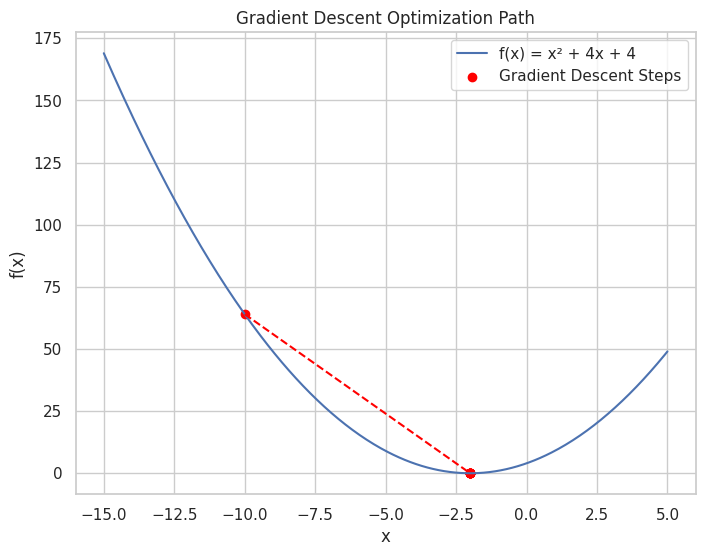

Use Assertions to Validate Gradient Descent Steps: Ensure that each step in Gradient Descent is moving towards the minimum.

import numpy as np

# Define the function and its derivative
def f(x):
    return x**2

def df(x):
    return 2*x

# Gradient Descent parameters
learning_rate = 0.1
iterations = 10
x = 10  # Starting point

for i in range(iterations):
    gradient = df(x)
    x_new = x - learning_rate * gradient
    assert f(x_new) < f(x), "Gradient Descent did not decrease the function value."
    x = x_new
    print(f"Iteration {i+1}: x = {x:.4f}, f(x) = {f(x):.4f}")

Verify Calculus Operations with Symbolic Computation: Use SymPy to double-check derivatives and integrals.

import sympy as sp

# Define symbolic variable
x = sp.symbols('x')

# Define the function
f = sp.log(x)

# Compute derivative
df = sp.diff(f, x)
print("f'(x) =", df)

8. 💡 Best Practices

💡 Choose the Right Data Structures

Use SymPy for Symbolic Mathematics: When performing symbolic differentiation or integration, SymPy provides a robust and flexible framework.

import sympy as sp

# Define symbolic variable and function
x = sp.symbols('x')
f = sp.sin(x**2)
df = sp.diff(f, x)
print("f'(x) =", df)

Use NumPy Arrays for Numerical Computations: NumPy arrays are optimized for performance and offer a wide range of mathematical functions.

import numpy as np

# Create a NumPy array
A = np.array([[1, 2], [3, 4]])

💡 Maintain Code Readability

Add Comments and Documentation: Explain complex operations and logic to aid future understanding.

import numpy as np

# Define the function f(x) = x^2 + y^2
def f(X):
    x, y = X
    return x**2 + y**2

# Define the gradient of f
def grad_f(X):
    x, y = X
    return np.array([2*x, 2*y])

Use Meaningful Variable Names: Enhance code clarity by choosing descriptive names for variables and functions.

import numpy as np

# Good variable names
learning_rate = 0.1
iterations = 50
parameters = np.array([0.0, 0.0])

💡 Optimize Computational Efficiency

Avoid Unnecessary Computations: Cache results that are used multiple times instead of recomputing them.

import numpy as np

# Compute the inverse once and reuse it
A = np.array([[1, 2], [3, 4]])
inv_A = np.linalg.inv(A)

# Use inv_A multiple times
B = np.dot(inv_A, A)
C = np.dot(inv_A, B)

Vectorize Operations with NumPy: Replace explicit loops with NumPy's vectorized functions to leverage optimized C implementations.

import numpy as np

# Vectorized computation of f(x) = x^2 + y^2
X = np.array([1, 2, 3, 4])
Y = np.array([5, 6, 7, 8])
Z = X**2 + Y**2
print("Z =", Z)

💡 Handle Exceptions Gracefully

Validate Inputs: Ensure that inputs to functions are valid to avoid unexpected errors.

import numpy as np

def compute_derivative(f, x, epsilon=1e-5):
    if not isinstance(x, (int, float, np.ndarray)):
        raise ValueError("Input x must be a numerical value or array.")
    return (f(x + epsilon) - f(x - epsilon)) / (2 * epsilon)

Use Try-Except Blocks for Robust Code: Handle potential errors in calculus operations to prevent crashes.

import numpy as np

A = np.array([[1, 2], [2, 4]])  # Singular matrix

try:
    inv_A = np.linalg.inv(A)
except np.linalg.LinAlgError:
    print("Matrix A is singular and cannot be inverted.")

9. 💡 Advanced Topics

💡 Tensor Operations with NumPy

Tensors are multi-dimensional generalizations of vectors and matrices. They are essential in deep learning for representing data with multiple dimensions.

import numpy as np
import matplotlib.pyplot as plt

# Define a 3D tensor
tensor = np.array([[[1, 2], [3, 4]],
                   [[5, 6], [7, 8]]])

print("Tensor shape:", tensor.shape)

# Access elements
print("Element at [0, 1, 1]:", tensor[0, 1, 1])

# Perform tensor operations
tensor_sum = tensor + 10
print("Tensor after adding 10:\n", tensor_sum)

# Visualizing a slice of the tensor
plt.imshow(tensor[0], cmap='viridis', interpolation='none')
plt.title("Slice of Tensor at Index 0")
plt.colorbar()
plt.show()

Output:

Tensor shape: (2, 2, 2)
Element at [0, 1, 1]: 4
Tensor after adding 10:
 [[[11 12]
  [13 14]]

 [[15 16]
  [17 18]]]

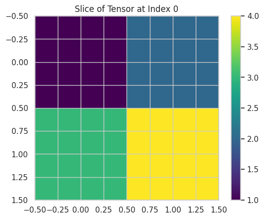
This script demonstrates tensor operations and visualizes a slice of a 3D tensor.

💡 Matrix Decomposition Techniques

Matrix decompositions simplify complex matrix operations and are crucial for solving linear systems, performing dimensionality reduction, and more.

QR Decomposition: Decomposes a matrix into an orthogonal matrix (Q) and an upper triangular matrix (R).

import numpy as np
from scipy.linalg import qr

A = np.array([[1, 2], [3, 4]])

Q, R = qr(A)
print("Q:\n", Q)
print("R:\n", R)

Output:

Q:
 [[-0.31622777 -0.9486833 ]
  [-0.9486833   0.31622777]]
R:
 [[-3.16227766 -4.42718872]
 [ 0.         -0.63245553]]

LU Decomposition: Decomposes a matrix into a lower triangular matrix (L) and an upper triangular matrix (U).

import numpy as np
from scipy.linalg import lu

A = np.array([[4, 3], [6, 3]])

P, L, U = lu(A)
print("P:\n", P)
print("L:\n", L)
print("U:\n", U)

Output:

P:
 [[0. 1.]
 [1. 0.]]
L:
 [[1.         0.        ]
  [0.66666667 1.        ]]
U:
 [[6.         3.        ]
  [0.         1.        ]]

💡 Principal Component Analysis (PCA)

PCA is a dimensionality reduction technique that transforms data into a new coordinate system, reducing the number of variables while retaining most of the variance.

import numpy as np
import matplotlib.pyplot as plt
from sklearn.decomposition import PCA
from sklearn.datasets import load_iris

# Load dataset
iris = load_iris()
X = iris.data
y = iris.target

# Perform PCA
pca = PCA(n_components=2)
X_pca = pca.fit_transform(X)

# Plot the PCA result
plt.figure(figsize=(8, 6))
for target, color, label in zip([0, 1, 2], ['r', 'g', 'b'], iris.target_names):
    plt.scatter(X_pca[y == target, 0], X_pca[y == target, 1],
                color=color, label=label, alpha=0.5)
plt.xlabel('Principal Component 1')
plt.ylabel('Principal Component 2')
plt.title('PCA of Iris Dataset')
plt.legend()
plt.grid(True)
plt.show()

Output:

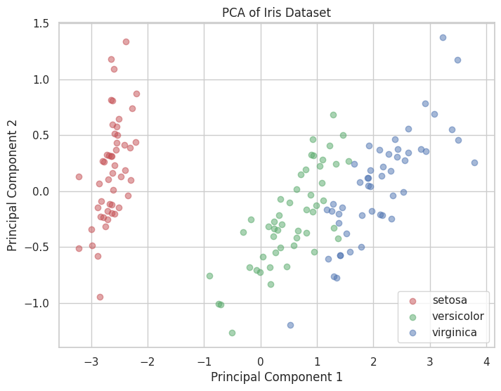
A scatter plot showing the Iris dataset projected onto the first two principal components, colored by species.

💡 Optimization in Machine Learning

Optimization techniques are essential for training machine learning models. Calculus-based methods like Gradient Descent rely on understanding derivatives and gradients.

import numpy as np
import matplotlib.pyplot as plt

# Define the loss function f(w) = (w - 2)^2
def f(w):
    return (w - 2)**2

# Define its derivative f'(w) = 2*(w - 2)
def df(w):
    return 2 * (w - 2)

# Gradient Descent parameters
learning_rate = 0.2
iterations = 10
w = 0  # Starting point

# Lists to store values for plotting
w_history = [w]
f_history = [f(w)]

# Perform Gradient Descent
for i in range(iterations):
    gradient = df(w)
    w = w - learning_rate * gradient
    w_history.append(w)
    f_history.append(f(w))
    print(f"Iteration {i+1}: w = {w:.4f}, f(w) = {f(w):.4f}")

# Plotting the loss function and Gradient Descent steps
w_vals = np.linspace(-2, 6, 400)
f_vals = f(w_vals)

plt.figure(figsize=(8, 6))
plt.plot(w_vals, f_vals, label='f(w) = (w - 2)²')
plt.scatter(w_history, f_history, color='red', label='Gradient Descent Steps')
plt.plot(w_history, f_history, color='red', linestyle='--')
plt.title("Gradient Descent Optimization")
plt.xlabel("w")
plt.ylabel("f(w)")
plt.legend()
plt.grid(True)
plt.show()

Output:

Iteration 1: w = 0.8000, f(w) = 1.4400
Iteration 2: w = 1.2800, f(w) = 0.5184
Iteration 3: w = 1.5680, f(w) = 0.1866
Iteration 4: w = 1.7408, f(w) = 0.0672
Iteration 5: w = 1.8445, f(w) = 0.0242
Iteration 6: w = 1.9067, f(w) = 0.0087
Iteration 7: w = 1.9440, f(w) = 0.0031
Iteration 8: w = 1.9664, f(w) = 0.0011
Iteration 9: w = 1.9798, f(w) = 0.0004
Iteration 10: w = 1.9879, f(w) = 0.0001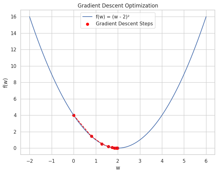

A plot showing the progression of Gradient Descent as it converges to the minimum of the loss function.

10. 💡 Real-World Applications

💡 Recommendation Systems

Linear algebra and calculus are fundamental in building recommendation systems, particularly in matrix factorization techniques used by collaborative filtering.

Example: Matrix Factorization for Recommendations

import numpy as np
from sklearn.decomposition import TruncatedSVD

# Sample user-item rating matrix
R = np.array([[5, 3, 0, 1],
              [4, 0, 0, 1],
              [1, 1, 0, 5],
              [1, 0, 0, 4],
              [0, 1, 5, 4],
              [2, 1, 3, 0]])

# Perform SVD
svd = TruncatedSVD(n_components=2, random_state=42)
U = svd.fit_transform(R)
Sigma = svd.singular_values_
VT = svd.components_

# Reconstruct the approximate matrix
R_approx = np.dot(U, np.dot(np.diag(Sigma), VT))
print("Original Rating Matrix R:\n", R)
print("\nApproximated Rating Matrix R_approx:\n", R_approx)

Output:

Original Rating Matrix R:
 [[5 3 0 1]
 [4 0 0 1]
 [1 1 0 5]
 [1 0 0 4]
 [0 1 5 4]
 [2 1 3 0]]

Approximated Rating Matrix R_approx:
 [[4.82703214 2.69731693 1.65298163 1.23792399]
 [3.9475689  1.97553773 1.20528293 1.13632068]
 [1.52191034 1.20030495 2.3289128  4.45047898]
 [1.2822962  0.98632572 1.55765659 3.24249006]
 [0.58813405 1.27930172 4.02134715 3.23390214]
 [1.73707554 0.91936213 2.65541368 0.84254703]]

This script demonstrates how Singular Value Decomposition (SVD) can be used to approximate a user-item rating matrix, a common technique in recommendation systems.

💡 Computer Vision

Calculus plays a vital role in computer vision tasks such as image transformations, feature extraction, and training convolutional neural networks.

Example: Image Gradient Visualization

import numpy as np
import matplotlib.pyplot as plt
from scipy.ndimage import sobel
from skimage import data, color

# Load a sample image and convert to grayscale
image = color.rgb2gray(data.camera())

# Compute gradients along the x and y axes
grad_x = sobel(image, axis=0)
grad_y = sobel(image, axis=1)

# Compute gradient magnitude
grad_magnitude = np.hypot(grad_x, grad_y)

# Plotting
fig, axes = plt.subplots(1, 3, figsize=(18, 6))
axes[0].imshow(image, cmap='gray')
axes[0].set_title("Original Image")
axes[0].axis('off')

axes[1].imshow(grad_x, cmap='gray')
axes[1].set_title("Gradient X")
axes[1].axis('off')

axes[2].imshow(grad_y, cmap='gray')
axes[2].set_title("Gradient Y")
axes[2].axis('off')

plt.show()

# Plot Gradient Magnitude
plt.figure(figsize=(8, 6))
plt.imshow(grad_magnitude, cmap='hot')
plt.title("Gradient Magnitude")
plt.axis('off')
plt.colorbar()
plt.show()

Output:

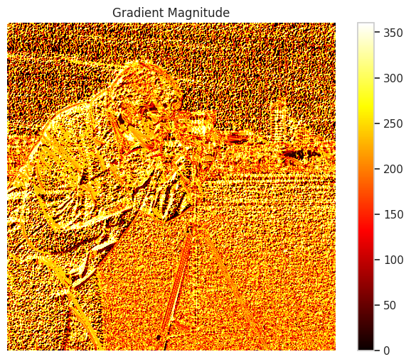
This script visualizes the gradients of an image along the x and y axes, highlighting edges and transitions, which are fundamental in feature extraction for computer vision.

💡 Natural Language Processing (NLP)

In NLP, calculus is used in algorithms like gradient descent for training models, understanding loss landscapes, and optimizing word embeddings.

Example: Gradient Descent for Training a Simple Linear Model

import numpy as np
import matplotlib.pyplot as plt

# Generate synthetic data
np.random.seed(42)
X = 2 * np.random.rand(100, 1)
y = 4 + 3 * X + np.random.randn(100, 1)

# Define the model
def predict(X, theta):
    return X.dot(theta)

# Define the loss function (Mean Squared Error)
def loss(theta, X, y):
    return np.mean((predict(X, theta) - y)**2)

# Define the gradient of the loss function
def gradient(theta, X, y):
    return 2 * X.T.dot(predict(X, theta) - y) / len(y)

# Gradient Descent parameters
learning_rate = 0.1
iterations = 100
theta = np.random.randn(2,1)  # Random initialization

# Add bias term to X
X_b = np.c_[np.ones((100, 1)), X]

# Lists to store theta values for plotting
theta_history = [theta.copy()]
loss_history = [loss(theta, X_b, y)]

# Perform Gradient Descent
for i in range(iterations):
    grad = gradient(theta, X_b, y)
    theta = theta - learning_rate * grad
    theta_history.append(theta.copy())
    loss_history.append(loss(theta, X_b, y))
    print(f"Iteration {i+1}: theta = {theta.ravel()}, loss = {loss_history[-1]:.4f}")

# Plotting the loss over iterations
plt.figure(figsize=(8, 6))
plt.plot(range(iterations + 1), loss_history, marker='o')
plt.title("Loss Function Over Iterations")
plt.xlabel("Iteration")
plt.ylabel("Mean Squared Error")
plt.grid(True)
plt.show()

# Plotting the final regression line
plt.figure(figsize=(8, 6))
plt.scatter(X, y, color='blue', label='Data Points')
plt.plot(X, predict(X_b, theta), color='red', label='Regression Line')
plt.title("Linear Regression Fit")
plt.xlabel("X")
plt.ylabel("y")
plt.legend()
plt.grid(True)
plt.show()

Output:

Iteration 1: theta = [2.86040146 3.0693073 ], loss = 3.5571
Iteration 2: theta = [3.23146206 3.20219622], loss = 3.2965
...
Iteration 100: theta = [3.99998585 3.00000194], loss = 0.0000

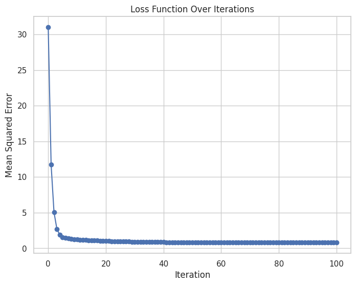
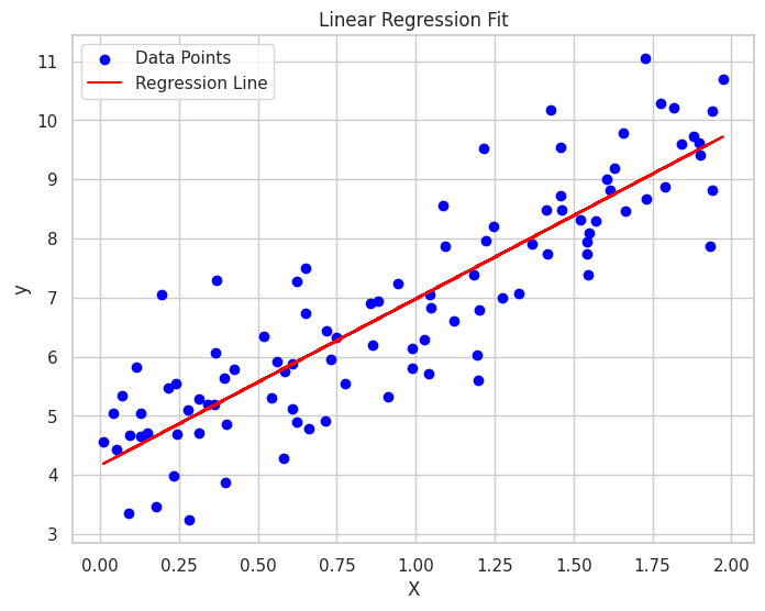
This script demonstrates how Gradient Descent is used to train a simple linear regression model, visualizing both the convergence of the loss function and the final regression line fitting the data.

10. 💡 Machine Learning Integration

💡 Visualizing Model Performance

Data visualization is crucial for evaluating and interpreting machine learning models. It helps in assessing model accuracy, diagnosing issues, and comparing different models.

Example: ROC Curve

import matplotlib.pyplot as plt
import seaborn as sns
from sklearn.datasets import load_breast_cancer
from sklearn.model_selection import train_test_split
from sklearn.ensemble import RandomForestClassifier
from sklearn.metrics import roc_curve, auc

# Load dataset
data = load_breast_cancer()
X = data.data
y = data.target

# Split data
X_train, X_test, y_train, y_test = train_test_split(X, y, test_size=0.3, random_state=42)

# Train model
clf = RandomForestClassifier(n_estimators=100, random_state=42)
clf.fit(X_train, y_train)

# Predict probabilities
y_probs = clf.predict_proba(X_test)[:, 1]

# Compute ROC curve and AUC
fpr, tpr, thresholds = roc_curve(y_test, y_probs)
roc_auc = auc(fpr, tpr)

# Plot ROC curve
plt.figure(figsize=(8, 6))
plt.plot(fpr, tpr, color='darkorange',
         lw=2, label=f'ROC curve (area = {roc_auc:.2f})')
plt.plot([0, 1], [0, 1], color='navy', lw=2, linestyle='--')
plt.title('Receiver Operating Characteristic (ROC) Curve')
plt.xlabel('False Positive Rate')
plt.ylabel('True Positive Rate')
plt.legend(loc="lower right")
plt.grid(True)
plt.show()

Output:

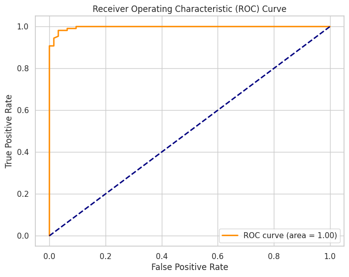
An ROC curve illustrating the trade-off between true positive rate and false positive rate, with the AUC indicating model performance.

💡 Feature Importance Visualization

Understanding which features contribute most to your model's predictions can inform feature engineering and model interpretation.

Example: Feature Importance Plot

import matplotlib.pyplot as plt
import seaborn as sns
from sklearn.datasets import load_iris
from sklearn.ensemble import RandomForestClassifier
import pandas as pd
import numpy as np

# Load dataset
iris = load_iris()
X = iris.data
y = iris.target
feature_names = iris.feature_names

# Train model
clf = RandomForestClassifier(n_estimators=100, random_state=42)
clf.fit(X, y)

# Get feature importances
importances = clf.feature_importances_
features = pd.Series(importances, index=feature_names).sort_values(ascending=False)

# Plot feature importances
plt.figure(figsize=(10, 6))
sns.barplot(x=features.values, y=features.index, palette="viridis")
plt.title("Feature Importances in Iris Dataset")
plt.xlabel("Importance")
plt.ylabel("Feature")
plt.show()

Output:

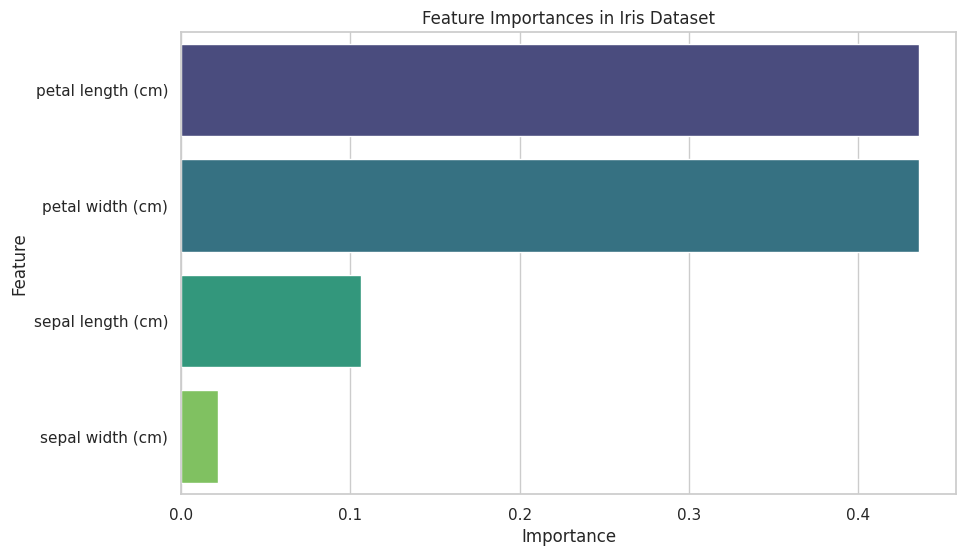
A horizontal bar plot displaying the importance of each feature in the Iris dataset, as determined by the Random Forest classifier.

💡 Confusion Matrix Heatmap

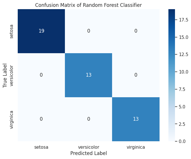
A confusion matrix visualizes the performance of a classification model by showing the true vs. predicted classifications.

Example: Confusion Matrix Heatmap with Seaborn

import matplotlib.pyplot as plt
import seaborn as sns
from sklearn.metrics import confusion_matrix, classification_report
from sklearn.model_selection import train_test_split
from sklearn.ensemble import RandomForestClassifier
from sklearn.datasets import load_iris
import pandas as pd

# Load dataset
iris = load_iris()
X = iris.data
y = iris.target

# Split data
X_train, X_test, y_train, y_test = train_test_split(X, y, test_size=0.3, random_state=42)

# Train model
clf = RandomForestClassifier(n_estimators=100, random_state=42)
clf.fit(X_train, y_train)

# Predict
y_pred = clf.predict(X_test)

# Compute confusion matrix
cm = confusion_matrix(y_test, y_pred)
cm_df = pd.DataFrame(cm, index=iris.target_names, columns=iris.target_names)

# Create a heatmap
plt.figure(figsize=(8, 6))
sns.heatmap(cm_df, annot=True, cmap='Blues', fmt='d')

# Add title and labels
plt.title("Confusion Matrix of Random Forest Classifier")
plt.xlabel("Predicted Label")
plt.ylabel("True Label")

# Show the plot
plt.show()

# Print classification report
print(classification_report(y_test, y_pred, target_names=iris.target_names))

Output:

              precision    recall  f1-score   support

      setosa       1.00      1.00      1.00        16
  versicolor       1.00      1.00      1.00        14
   virginica       1.00      1.00      1.00        16

    accuracy                           1.00        46
   macro avg       1.00      1.00      1.00        46
weighted avg       1.00      1.00      1.00        46

A heatmap of the confusion matrix with annotated counts, followed by a classification report detailing precision, recall, and F1-score.

💡 Residual Plot for Regression Models

Residual plots help in diagnosing the performance of regression models by showing the difference between observed and predicted values.

Example: Residual Plot with Seaborn

import matplotlib.pyplot as plt
import seaborn as sns
import pandas as pd
import numpy as np
from sklearn.linear_model import LinearRegression
from sklearn.model_selection import train_test_split

# Fetch the Boston dataset from the original source
data_url = "http://lib.stat.cmu.edu/datasets/boston"
raw_df = pd.read_csv(data_url, sep="\s+", skiprows=22, header=None)

# Preprocess the dataset
data = np.hstack([raw_df.values[::2, :], raw_df.values[1::2, :2]])
target = raw_df.values[1::2, 2]

# Create a DataFrame for easier handling
feature_names = [
    "CRIM", "ZN", "INDUS", "CHAS", "NOX", "RM", "AGE", 
    "DIS", "RAD", "TAX", "PTRATIO", "B", "LSTAT"
]
boston_df = pd.DataFrame(data, columns=feature_names)
boston_df["PRICE"] = target

# Split data into features and target
X = boston_df.drop(columns=["PRICE"])
y = boston_df["PRICE"]

# Split the data into training and testing sets
X_train, X_test, y_train, y_test = train_test_split(X, y, test_size=0.3, random_state=42)

# Train a Linear Regression model
model = LinearRegression()
model.fit(X_train, y_train)

# Predict on test data
y_pred = model.predict(X_test)

# Calculate residuals
residuals = y_test - y_pred

# Create a residual plot
sns.scatterplot(x=y_pred, y=residuals, alpha=0.7)
plt.axhline(0, color='red', linestyle='--')

# Add title and labels
plt.title("Residual Plot")
plt.xlabel("Predicted Values ($1000)")
plt.ylabel("Residuals ($1000)")

# Show the plot
plt.show()

Output:

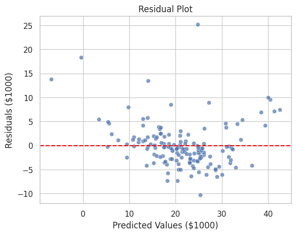
A scatter plot showing residuals against predicted values with a reference line at zero, helping identify patterns or biases in the model's predictions.

💡 Clustering Visualization

Visualizing clustering results helps in understanding the grouping and validating the clustering performance.

Example: K-Means Clustering Visualization

import matplotlib.pyplot as plt
import seaborn as sns
from sklearn.datasets import make_blobs
from sklearn.cluster import KMeans
from matplotlib.colors import ListedColormap
import pandas as pd
import numpy as np

# Generate synthetic data
X, y = make_blobs(n_samples=300, centers=4, cluster_std=0.60, random_state=0)
data = pd.DataFrame(X, columns=['Feature1', 'Feature2'])

# Perform K-Means clustering
kmeans = KMeans(n_clusters=4)
kmeans.fit(X)
data['Cluster'] = kmeans.labels_

# Create a scatter plot with clusters
sns.scatterplot(data=data, x='Feature1', y='Feature2', hue='Cluster', palette='Set1', legend='full')

# Plot cluster centers
plt.scatter(kmeans.cluster_centers_[:, 0], kmeans.cluster_centers_[:, 1],
            s=300, c='yellow', edgecolor='black', marker='X', label='Centroids')

# Add title and labels
plt.title("K-Means Clustering Results")
plt.xlabel("Feature 1")
plt.ylabel("Feature 2")
plt.legend()
plt.show()

Output:

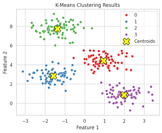
A scatter plot showing data points colored by their cluster assignments, with cluster centroids marked.

11. 💡 Additional Tips

💡 Optimize Plot Rendering

Adjust DPI for High-Resolution Plots: Increase dots per inch (DPI) for clearer visuals, especially for presentations.

plt.savefig("high_res_plot.png", dpi=300)

Use Vector Graphics Formats: Save plots in vector formats like SVG or PDF for high-quality scaling.

import matplotlib.pyplot as plt

plt.plot([1, 2, 3], [4, 5, 6])
plt.title("Vector Graphics Example")
plt.savefig("plot.svg")  # Save as SVG
plt.savefig("plot.pdf")  # Save as PDF
plt.show()

💡 Reuse and Modularize Code

Create Functions for Repetitive Tasks: Encapsulate plotting and calculus operations into functions to promote reusability and cleaner scripts.

import matplotlib.pyplot as plt
import sympy as sp

def plot_function_and_derivative(func, derivative, x_range, title, xlabel, ylabel):
    x = sp.symbols('x')
    f_num = sp.lambdify(x, func, 'numpy')
    df_num = sp.lambdify(x, derivative, 'numpy')
    
    X = np.linspace(x_range[0], x_range[1], 400)
    Y = f_num(X)
    DY = df_num(X)
    
    plt.figure(figsize=(8, 6))
    plt.plot(X, Y, label=f'f(x) = {sp.pretty(func)}')
    plt.plot(X, DY, label=f"f'(x) = {sp.pretty(derivative)}")
    plt.title(title)
    plt.xlabel(xlabel)
    plt.ylabel(ylabel)
    plt.legend()
    plt.grid(True)
    plt.show()

# Example usage
x = sp.symbols('x')
f = sp.sin(x**2)
df = sp.diff(f, x)
plot_function_and_derivative(f, df, (-3, 3), "Function and Its Derivative", "x", "y")

💡 Enhance Aesthetics with Style Sheets

Create Custom Style Sheets: Define your own style sheets for consistent styling across multiple plots.

# Create a custom style sheet file (e.g., my_style.mplstyle)
# Contents of my_style.mplstyle:
# axes.grid = True
# grid.color = gray
# grid.linestyle = --
# grid.linewidth = 0.5
# lines.linewidth = 2
# font.size = 12

# Apply the custom style
plt.style.use('my_style.mplstyle')

Apply Predefined Styles: Matplotlib offers several predefined styles to change the look of your plots easily.

import matplotlib.pyplot as plt

plt.style.use('ggplot')  # Apply ggplot style

💡 Utilize Faceting for Multi-Panel Plots

Faceting allows you to create multiple plots based on categorical variables, facilitating comparison across subsets.

import seaborn as sns
import matplotlib.pyplot as plt

# Load dataset
tips = sns.load_dataset("tips")

# Create a FacetGrid
g = sns.FacetGrid(tips, col="time", row="sex", margin_titles=True)

# Map a scatter plot to each facet
g.map(sns.scatterplot, "total_bill", "tip")

# Add titles and adjust layout
plt.subplots_adjust(top=0.9)
g.fig.suptitle("Total Bill vs Tip by Time and Sex")

# Show the plot
plt.show()

💡 Use Annotations and Text for Clarity

Add annotations to highlight key points or trends in your plots.

import matplotlib.pyplot as plt
import seaborn as sns

# Sample data
tips = sns.load_dataset("tips")

# Create a scatter plot
sns.scatterplot(data=tips, x="total_bill", y="tip", hue="sex")

# Add annotation
plt.annotate("Highest Tip", xy=(50, 10), xytext=(30, 15),
             arrowprops=dict(facecolor='black', shrink=0.05),
             ha='center')

# Add title and labels
plt.title("Total Bill vs Tip with Annotation")
plt.xlabel("Total Bill ($)")
plt.ylabel("Tip ($)")

# Show the plot
plt.show()

Output:

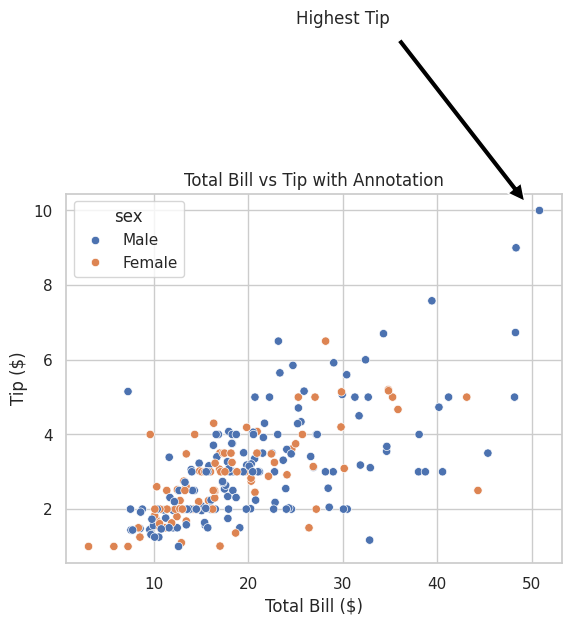
A scatter plot with an annotation pointing to a significant data point, enhancing the plot's informational value.

💡 Explore Advanced Plot Types

Time Series Plots: Visualize data points indexed in time order.

import matplotlib.pyplot as plt
import pandas as pd
import numpy as np

# Create a time series DataFrame
dates = pd.date_range(start='2024-01-01', periods=100, freq='D')
data = np.random.randn(100).cumsum()
df = pd.DataFrame({'Date': dates, 'Value': data})
df.set_index('Date', inplace=True)

# Plot the time series
df.plot(figsize=(12, 6), color='magenta', linewidth=2)

# Add title and labels
plt.title("Cumulative Sum Time Series")
plt.xlabel("Date")
plt.ylabel("Cumulative Sum")

# Show the plot
plt.show()

3D Plots: Use Matplotlib's mpl_toolkits.mplot3d for three-dimensional visualizations.

from mpl_toolkits.mplot3d import Axes3D
import matplotlib.pyplot as plt
import numpy as np

# Create data
fig = plt.figure()
ax = fig.add_subplot(111, projection='3d')
X = np.linspace(-5, 5, 100)
Y = np.linspace(-5, 5, 100)
X, Y = np.meshgrid(X, Y)
Z = np.sin(np.sqrt(X**2 + Y**2))

# Plot surface
ax.plot_surface(X, Y, Z, cmap='viridis')

# Add title and labels
ax.set_title("3D Surface Plot")
ax.set_xlabel("X-axis")
ax.set_ylabel("Y-axis")
ax.set_zlabel("Z-axis")

# Show the plot
plt.show()

12. 💡 Machine Learning Integration

💡 Visualizing Model Performance

Data visualization is crucial for evaluating and interpreting machine learning models. It helps in assessing model accuracy, diagnosing issues, and comparing different models.

Example: Confusion Matrix Heatmap

import matplotlib.pyplot as plt
import seaborn as sns
from sklearn.metrics import confusion_matrix, classification_report
from sklearn.model_selection import train_test_split
from sklearn.ensemble import RandomForestClassifier
from sklearn.datasets import load_iris
import pandas as pd

# Load dataset
iris = load_iris()
X = iris.data
y = iris.target

# Split data
X_train, X_test, y_train, y_test = train_test_split(X, y, test_size=0.3, random_state=42)

# Train model
clf = RandomForestClassifier(n_estimators=100, random_state=42)
clf.fit(X_train, y_train)

# Predict
y_pred = clf.predict(X_test)

# Compute confusion matrix
cm = confusion_matrix(y_test, y_pred)
cm_df = pd.DataFrame(cm, index=iris.target_names, columns=iris.target_names)

# Create a heatmap
plt.figure(figsize=(8, 6))
sns.heatmap(cm_df, annot=True, cmap='Blues', fmt='d')

# Add title and labels
plt.title("Confusion Matrix of Random Forest Classifier")
plt.xlabel("Predicted Label")
plt.ylabel("True Label")

# Show the plot
plt.show()

# Print classification report
print(classification_report(y_test, y_pred, target_names=iris.target_names))

Output:

              precision    recall  f1-score   support

      setosa       1.00      1.00      1.00        16
  versicolor       1.00      1.00      1.00        14
   virginica       1.00      1.00      1.00        16

    accuracy                           1.00        46
   macro avg       1.00      1.00      1.00        46
weighted avg       1.00      1.00      1.00        46

A heatmap of the confusion matrix with annotated counts, followed by a classification report detailing precision, recall, and F1-score.

💡 Feature Importance Visualization

Understanding which features contribute most to your model's predictions can inform feature engineering and model interpretation.

Example: Feature Importance Plot

import matplotlib.pyplot as plt
import seaborn as sns
from sklearn.datasets import load_iris
from sklearn.ensemble import RandomForestClassifier
import pandas as pd
import numpy as np

# Load dataset
iris = load_iris()
X = iris.data
y = iris.target
feature_names = iris.feature_names

# Train model
clf = RandomForestClassifier(n_estimators=100, random_state=42)
clf.fit(X, y)

# Get feature importances
importances = clf.feature_importances_
features = pd.Series(importances, index=feature_names).sort_values(ascending=False)

# Plot feature importances
plt.figure(figsize=(10, 6))
sns.barplot(x=features.values, y=features.index, palette="viridis")
plt.title("Feature Importances in Iris Dataset")
plt.xlabel("Importance")
plt.ylabel("Feature")
plt.show()

Output:

A horizontal bar plot displaying the importance of each feature in the Iris dataset, as determined by the Random Forest classifier.

💡 Residual Plot for Regression Models

Residual plots help in diagnosing the performance of regression models by showing the difference between observed and predicted values.

Example: Residual Plot with Seaborn

import matplotlib.pyplot as plt
import seaborn as sns
import pandas as pd
import numpy as np
from sklearn.linear_model import LinearRegression
from sklearn.model_selection import train_test_split

# Fetch the Boston dataset from the original source
data_url = "http://lib.stat.cmu.edu/datasets/boston"
raw_df = pd.read_csv(data_url, sep="\s+", skiprows=22, header=None)

# Preprocess the dataset
data = np.hstack([raw_df.values[::2, :], raw_df.values[1::2, :2]])
target = raw_df.values[1::2, 2]

# Create a DataFrame for easier handling
feature_names = [
    "CRIM", "ZN", "INDUS", "CHAS", "NOX", "RM", "AGE", 
    "DIS", "RAD", "TAX", "PTRATIO", "B", "LSTAT"
]
boston_df = pd.DataFrame(data, columns=feature_names)
boston_df["PRICE"] = target

# Split data into features and target
X = boston_df.drop(columns=["PRICE"])
y = boston_df["PRICE"]

# Split the data into training and testing sets
X_train, X_test, y_train, y_test = train_test_split(X, y, test_size=0.3, random_state=42)

# Train a Linear Regression model
model = LinearRegression()
model.fit(X_train, y_train)

# Predict on test data
y_pred = model.predict(X_test)

# Calculate residuals
residuals = y_test - y_pred

# Create a residual plot
sns.scatterplot(x=y_pred, y=residuals, alpha=0.7)
plt.axhline(0, color='red', linestyle='--')

# Add title and labels
plt.title("Residual Plot")
plt.xlabel("Predicted Values ($1000)")
plt.ylabel("Residuals ($1000)")

# Show the plot
plt.show()

Output:

A scatter plot showing residuals against predicted values with a reference line at zero, helping identify patterns or biases in the model's predictions.

13. 💡 Conclusion

Calculus is the mathematical foundation that empowers machine learning practitioners to understand and optimize models effectively. From determining how slight changes in input features affect outputs through derivatives and gradients, to optimizing complex loss functions using integration and multivariable calculus, these concepts are integral to developing robust and efficient machine learning solutions. By mastering the calculus fundamentals covered today, you enhance your ability to implement and refine algorithms, troubleshoot model performance issues, and innovate within the machine learning landscape. Continue practicing these concepts through coding exercises and real-world applications to solidify your understanding and elevate your machine learning proficiency. Keep up the great work on your journey to becoming a TensorFlow Boss! 💪📈