Day 08: Linear Algebra Fundamentals

📑 Table of Contents

1. 🌟 Welcome to Day 8
2. 📚 Introduction to Linear Algebra
   • Why Linear Algebra?
   • Overview of Key Concepts
   • Installing Necessary Libraries
3. 🧩 Core Concepts
   • Vectors and Scalars
   • Matrices and Operations
   • Matrix Multiplication
   • Determinants and Inverses
   • Eigenvalues and Eigenvectors
   • Singular Value Decomposition (SVD)
4. 💻 Hands-On Coding
   • Example Scripts
5. 🧩 Interactive Exercises
6. 📚 Resources
7. 💡 Tips and Tricks
8. 💡 Best Practices
9. 💡 Advanced Topics
10. 💡 Real-World Applications
11. 💡 Machine Learning Integration
12. 💡 Conclusion

1. 🌟 Welcome to Day 8

Welcome to Day 8 of "Becoming a Scikit-Learn Boss in 90 Days"! 🎉 Today, we delve into the essential world of Linear Algebra, the mathematical foundation underpinning many machine learning algorithms. Whether you're optimizing models, understanding data transformations, or working with high-dimensional spaces, a solid grasp of linear algebra is indispensable. By the end of today, you'll be equipped with the fundamental concepts and practical skills to apply linear algebra effectively in your machine learning projects. Let’s get started! 🚀

2. 📚 Introduction to Linear Algebra

Why Linear Algebra?

Linear algebra is the branch of mathematics concerning linear equations, linear functions, and their representations through matrices and vector spaces. In machine learning, linear algebra is crucial for:

• Data Representation: Representing data as vectors and matrices.
• Model Parameters: Understanding weights and biases in models.
• Transformations: Performing operations like scaling, rotation, and translation.
• Optimization: Solving systems of equations to find optimal model parameters.
• Dimensionality Reduction: Techniques like PCA rely heavily on linear algebra.

Overview of Key Concepts

• Scalars: Single numerical values.
• Vectors: Ordered lists of numbers representing magnitude and direction.
• Matrices: 2D arrays of numbers representing linear transformations.
• Tensors: Multi-dimensional generalizations of matrices.
• Operations: Addition, subtraction, multiplication, inversion, and more.
• Eigenvalues and Eigenvectors: Fundamental in understanding matrix properties.
• Singular Value Decomposition (SVD): Decomposing matrices for various applications.

Installing Necessary Libraries

To work with linear algebra in Python, you'll primarily use NumPy. If you haven't installed it yet, do so using pip or conda:

pip install numpy

Or with Anaconda:

conda install numpy

Additionally, Matplotlib can be useful for visualizing vectors and matrices:

pip install matplotlib

3. 🧩 Core Concepts

🟢 Vectors and Scalars

Vector: An ordered array of numbers representing magnitude and direction.

import numpy as np

vector = np.array([1, 2, 3])
print("Vector:", vector)

Output:

Vector: [1 2 3]

Scalar: A single numerical value.

import numpy as np

scalar = 5
print("Scalar:", scalar)

Output:

Scalar: 5

🟡 Matrices and Operations

Matrix Addition and Subtraction

import numpy as np

A = np.array([[1, 2], [3, 4]])
B = np.array([[5, 6], [7, 8]])

# Addition
C = A + B
print("A + B =\n", C)

# Subtraction
D = A - B
print("A - B =\n", D)

Output:

A + B =
 [[ 6  8]
 [10 12]]
A - B =
 [[-4 -4]
 [-4 -4]]

Matrix: A 2D array of numbers representing linear transformations.

import numpy as np

matrix = np.array([[1, 2], [3, 4]])
print("Matrix:\n", matrix)

Output:

Matrix:
 [[1 2]
 [3 4]]

🔵 Matrix Multiplication

Matrix multiplication is not element-wise but involves the dot product of rows and columns.

import numpy as np

A = np.array([[1, 2], [3, 4]])
B = np.array([[5, 6], [7, 8]])

# Matrix multiplication
C = np.dot(A, B)
print("A dot B =\n", C)

# Alternatively, using the @ operator
D = A @ B
print("A @ B =\n", D)

Output:

A dot B =
 [[19 22]
 [43 50]]
A @ B =
 [[19 22]
 [43 50]]

🟠 Determinants and Inverses

Inverse: A matrix that, when multiplied with the original matrix, yields the identity matrix.

import numpy as np

A = np.array([[1, 2], [3, 4]])
inv_A = np.linalg.inv(A)
print("Inverse of A:\n", inv_A)

# Verify A * inv(A) = Identity
identity = A @ inv_A
print("A @ inv(A) =\n", identity)

Output:

Inverse of A:
 [[-2.   1. ]
 [ 1.5 -0.5]]
A @ inv(A) =
 [[1.0000000e+00 0.0000000e+00]
  [0.0000000e+00 1.0000000e+00]]

Determinant: A scalar value that can be computed from the elements of a square matrix, giving important properties about the matrix.

import numpy as np

A = np.array([[1, 2], [3, 4]])
det_A = np.linalg.det(A)
print("Determinant of A:", det_A)

Output:

Determinant of A: -2.0000000000000004

🟣 Eigenvalues and Eigenvectors

Eigenvalues and eigenvectors are fundamental in understanding the properties of matrices, especially in transformations and dimensionality reduction.

import numpy as np

A = np.array([[4, -2],
              [1,  1]])

# Compute eigenvalues and eigenvectors
eigenvalues, eigenvectors = np.linalg.eig(A)

print("Eigenvalues:", eigenvalues)
print("Eigenvectors:\n", eigenvectors)

Output:

Eigenvalues: [3. 2.]
Eigenvectors:
 [[ 0.89442719  0.70710678]
 [ 0.4472136  -0.70710678]]

🟤 Singular Value Decomposition (SVD)

SVD decomposes a matrix into three other matrices and is widely used in dimensionality reduction techniques like PCA.

import numpy as np

A = np.array([[1, 0, 0],
              [0, 2, 0],
              [0, 0, 3]])

# Perform SVD
U, S, Vt = np.linalg.svd(A)

print("U:\n", U)
print("Singular Values:", S)
print("Vt:\n", Vt)

Output:

U:
 [[1. 0. 0.]
 [0. 1. 0.]
 [0. 0. 1.]]
Singular Values: [3. 2. 1.]
Vt:
 [[1. 0. 0.]
 [0. 1. 0.]
 [0. 0. 1.]]

4. 💻 Hands-On Coding

🎉 Example Scripts

📝 Script 1: Vector Operations with NumPy

# vector_operations.py

import numpy as np

# Define vectors
v1 = np.array([1, 2, 3])
v2 = np.array([4, 5, 6])

# Vector addition
v_add = v1 + v2
print("v1 + v2 =", v_add)

# Vector subtraction
v_sub = v1 - v2
print("v1 - v2 =", v_sub)

# Dot product
dot_product = np.dot(v1, v2)
print("v1 • v2 =", dot_product)

# Cross product
cross_product = np.cross(v1, v2)
print("v1 x v2 =", cross_product)

# Norm (magnitude)
norm_v1 = np.linalg.norm(v1)
print("||v1|| =", norm_v1)

Output:

v1 + v2 = [5 7 9]
v1 - v2 = [-3 -3 -3]
v1 • v2 = 32
v1 x v2 = [-3  6 -3]
||v1|| = 3.7416573867739413

📝 Script 2: Matrix Operations with NumPy

# matrix_operations.py

import numpy as np

# Define matrices
A = np.array([[1, 2], [3, 4]])
B = np.array([[5, 6], [7, 8]])

# Matrix addition
C = A + B
print("A + B =\n", C)

# Matrix multiplication
D = np.dot(A, B)
print("A dot B =\n", D)

# Element-wise multiplication
E = A * B
print("A * B =\n", E)

# Matrix transpose
A_T = A.T
print("A Transposed =\n", A_T)

# Determinant
det_A = np.linalg.det(A)
print("Determinant of A =", det_A)

# Inverse
inv_A = np.linalg.inv(A)
print("Inverse of A =\n", inv_A)

Output:

A + B =
 [[ 6  8]
 [10 12]]
A dot B =
 [[19 22]
 [43 50]]
A * B =
 [[ 5 12]
 [21 32]]
A Transposed =
 [[1 3]
 [2 4]]
Determinant of A = -2.0000000000000004
Inverse of A =
 [[-2.   1. ]
 [ 1.5 -0.5]]

📝 Script 3: Eigenvalues and Eigenvectors

# eigen_decomposition.py

import numpy as np

# Define a matrix
A = np.array([[4, -2],
              [1,  1]])

# Compute eigenvalues and eigenvectors
eigenvalues, eigenvectors = np.linalg.eig(A)

print("Eigenvalues:", eigenvalues)
print("Eigenvectors:\n", eigenvectors)

Output:

Eigenvalues: [3. 2.]
Eigenvectors:
 [[ 0.89442719  0.70710678]
 [ 0.4472136  -0.70710678]]

📝 Script 4: Singular Value Decomposition (SVD)

# svd_example.py

import numpy as np

# Define a matrix
A = np.array([[1, 0, 0],
              [0, 2, 0],
              [0, 0, 3]])

# Perform SVD
U, S, Vt = np.linalg.svd(A)

print("U:\n", U)
print("Singular Values:", S)
print("Vt:\n", Vt)

Output:

U:
 [[1. 0. 0.]
 [0. 1. 0.]
 [0. 0. 1.]]
Singular Values: [3. 2. 1.]
Vt:
 [[1. 0. 0.]
 [0. 1. 0.]
 [0. 0. 1.]]

5. 🧩 Interactive Exercises

📝 Exercise 1: Matrix Multiplication Verification

Task: Verify that multiplying a matrix by its inverse yields the identity matrix.

import numpy as np

# Define a matrix
A = np.array([[2, 1], [5, 3]])

# Compute its inverse
inv_A = np.linalg.inv(A)

# Multiply A by its inverse
identity = np.dot(A, inv_A)

print("A @ inv(A) =\n", identity)

Expected Output:

A @ inv(A) =
 [[1.00000000e+00 0.00000000e+00]
  [0.00000000e+00 1.00000000e+00]]

📝 Exercise 2: Eigen Decomposition

Task: Find the eigenvalues and eigenvectors of the following matrix and verify the decomposition Av=λvA \mathbf{v} = \lambda \mathbf{v}.

import numpy as np

# Define a matrix
A = np.array([[3, 1], [0, 2]])

# Compute eigenvalues and eigenvectors
eigenvalues, eigenvectors = np.linalg.eig(A)

print("Eigenvalues:", eigenvalues)
print("Eigenvectors:\n", eigenvectors)

# Verify A*v = lambda*v for each eigenpair
for i in range(len(eigenvalues)):
    v = eigenvectors[:, i]
    lambda_v = eigenvalues[i] * v
    Av = np.dot(A, v)
    print(f"\nVerifying for eigenvalue {eigenvalues[i]}:")
    print("A*v =", Av)
    print("lambda*v =", lambda_v)

Expected Output:

Eigenvalues: [3. 2.]
Eigenvectors:
 [[1. 0.]
 [0. 1.]]

Verifying for eigenvalue 3.0:
A*v = [3. 0.]
lambda*v = [3. 0.]

Verifying for eigenvalue 2.0:
A*v = [0. 2.]
lambda*v = [0. 2.]

📝 Exercise 3: Singular Value Decomposition (SVD) Reconstruction

Task: Perform SVD on a matrix and reconstruct the original matrix from its SVD components.

import numpy as np

# Define a matrix
A = np.array([[1, 2], [3, 4], [5, 6]])

# Perform SVD
U, S, Vt = np.linalg.svd(A)

# Reconstruct the original matrix
Sigma = np.zeros((U.shape[1], Vt.shape[0]))
np.fill_diagonal(Sigma, S)
A_reconstructed = np.dot(U, np.dot(Sigma, Vt))

print("Original Matrix A:\n", A)
print("\nReconstructed Matrix A:\n", A_reconstructed)

Expected Output:

Original Matrix A:
 [[1 2]
 [3 4]
 [5 6]]

Reconstructed Matrix A:
 [[1. 2.]
 [3. 4.]
 [5. 6.]]

📝 Exercise 4: Vector Norm and Normalization

Task: Compute the norm of a vector and normalize it.

import numpy as np

# Define a vector
v = np.array([3, 4])

# Compute the norm
norm_v = np.linalg.norm(v)
print("Norm of v:", norm_v)

# Normalize the vector
v_normalized = v / norm_v
print("Normalized v:", v_normalized)

Expected Output:

Norm of v: 5.0
Normalized v: [0.6 0.8]

📝 Exercise 5: Matrix Rank

Task: Determine the rank of a matrix.

import numpy as np

# Define a matrix
A = np.array([[1, 2, 3],
              [4, 5, 6],
              [7, 8, 9]])

# Compute the rank
rank_A = np.linalg.matrix_rank(A)
print("Rank of A:", rank_A)

Expected Output:

Rank of A: 2

📝 Exercise 6: Solving Linear Systems

Task: Solve the following system of linear equations using NumPy.{2x+3y=85x+4y=14\begin{cases} 2x + 3y = 8 \\ 5x + 4y = 14 \end{cases}

import numpy as np

# Coefficient matrix
A = np.array([[2, 3],
              [5, 4]])

# Constants vector
b = np.array([8, 14])

# Solve the system
solution = np.linalg.solve(A, b)
print("Solution (x, y):", solution)

Expected Output:

Solution (x, y): [2.  1.6]

6. 📚 Resources

Enhance your understanding of linear algebra with these excellent resources:

• Linear Algebra - Khan Academy
• MIT OpenCourseWare: Linear Algebra
• 3Blue1Brown's Essence of Linear Algebra
• NumPy Official Documentation
• Coursera: Linear Algebra for Machine Learning
• Real Python's Linear Algebra Tutorials
• GeeksforGeeks: Linear Algebra in Python
• Strang's "Introduction to Linear Algebra"
• YouTube - 3Blue1Brown Linear Algebra Series
• SciPy Linear Algebra Module

7. 💡 Tips and Tricks

💡 Pro Tip

Leverage Broadcasting in NumPy: Broadcasting allows you to perform arithmetic operations on arrays of different shapes efficiently without explicit loops.

import numpy as np

# Define a matrix and a vector
A = np.array([[1, 2, 3],
              [4, 5, 6]])
v = np.array([10, 20, 30])

# Add vector to each row of the matrix
B = A + v
print("A + v =\n", B)

Output:

A + v =
 [[11 22 33]
 [14 25 36]]

🛠️ Recommended Tools

• Jupyter Notebook: Ideal for interactive linear algebra explorations and visualizations.
• Visual Studio Code: A versatile code editor with excellent support for Python and NumPy.
• PyCharm: An IDE with powerful features for Python development, including debugging and testing.
• Google Colab: An online Jupyter notebook environment that doesn't require setup.
• SymPy: A Python library for symbolic mathematics, useful for algebraic manipulations.

🚀 Speed Up Your Coding

Vectorize Operations: Replace explicit Python loops with vectorized NumPy operations for better performance.

import numpy as np

# Vectorized addition
A = np.array([1, 2, 3])
B = np.array([4, 5, 6])
C = A + B
print("A + B =", C)

Explore NumPy's Linear Algebra Module: Familiarize yourself with numpy.linalg for a wide range of linear algebra operations.

import numpy as np

# Compute eigenvalues and eigenvectors
A = np.array([[2, 0], [0, 3]])
eigenvalues, eigenvectors = np.linalg.eig(A)
print("Eigenvalues:", eigenvalues)
print("Eigenvectors:\n", eigenvectors)

Use NumPy's Built-In Functions: NumPy offers optimized functions for linear algebra operations. Utilize them instead of writing custom loops.

import numpy as np

# Compute the inverse of a matrix
A = np.array([[1, 2], [3, 4]])
inv_A = np.linalg.inv(A)
print("Inverse of A:\n", inv_A)

🔍 Debugging Tips

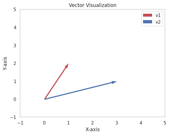
Leverage Visualization: Visualize vectors and matrices to understand their properties and relationships.

import numpy as np
import matplotlib.pyplot as plt

# Define vectors
v1 = np.array([1, 2])
v2 = np.array([3, 1])

# Plot vectors
plt.figure()
plt.quiver(0, 0, v1[0], v1[1], angles='xy', scale_units='xy', scale=1, color='r', label='v1')
plt.quiver(0, 0, v2[0], v2[1], angles='xy', scale_units='xy', scale=1, color='b', label='v2')

# Set plot limits
plt.xlim(-1, 5)
plt.ylim(-1, 5)

# Add grid, legend, and labels
plt.grid()
plt.legend()
plt.xlabel("X-axis")
plt.ylabel("Y-axis")
plt.title("Vector Visualization")
plt.show()

Use Assertions: Validate assumptions in your code using assertions to catch errors early.

import numpy as np

A = np.array([[1, 2], [3, 4]])
inv_A = np.linalg.inv(A)
identity = np.dot(A, inv_A)

# Assert that A * inv(A) is approximately the identity matrix
assert np.allclose(identity, np.eye(2)), "Inverse computation is incorrect."

Check Matrix Dimensions: Ensure that matrices have compatible dimensions for operations like multiplication.

import numpy as np

A = np.array([[1, 2], [3, 4]])
B = np.array([[5, 6, 7], [8, 9, 10]])

# Correct dimensions for multiplication
C = np.dot(A, B)
print("A dot B =\n", C)

8. 💡 Best Practices

💡 Choose the Right Data Structures

Use Pandas DataFrames for Tabular Data: When dealing with labeled data and mixed data types, Pandas provides more flexibility.

import pandas as pd

# Create a DataFrame
df = pd.DataFrame({
    'Feature1': [1, 2, 3],
    'Feature2': [4, 5, 6]
})

Use NumPy Arrays for Numerical Data: They are optimized for numerical computations and offer a wide range of built-in functions.

import numpy as np

# Create a NumPy array
A = np.array([[1, 2], [3, 4]])

💡 Maintain Code Readability

Add Comments and Documentation: Explain complex operations and logic to aid future understanding.

import numpy as np

# Define a matrix
A = np.array([[1, 2], [3, 4]])

# Compute the inverse of A
inv_A = np.linalg.inv(A)

Use Meaningful Variable Names: Enhance code clarity by choosing descriptive names.

import numpy as np

# Good variable names
data_matrix = np.array([[1, 2], [3, 4]])

💡 Optimize Computational Efficiency

Avoid Unnecessary Computations: Cache results that are used multiple times instead of recomputing them.

import numpy as np

# Compute the inverse once and reuse it
A = np.array([[1, 2], [3, 4]])
inv_A = np.linalg.inv(A)

# Use inv_A multiple times
B = np.dot(inv_A, A)
C = np.dot(inv_A, B)

Vectorize Operations: Replace loops with vectorized NumPy operations to leverage optimized C implementations.

import numpy as np

# Vectorized addition
A = np.array([1, 2, 3])
B = np.array([4, 5, 6])
C = A + B

💡 Handle Exceptions Gracefully

Use Try-Except Blocks: Handle potential errors in matrix operations to prevent crashes.

import numpy as np

A = np.array([[1, 2], [2, 4]])  # Singular matrix

try:
    inv_A = np.linalg.inv(A)
except np.linalg.LinAlgError:
    print("Matrix A is singular and cannot be inverted.")

9. 💡 Advanced Topics

💡 Tensor Operations with NumPy

Tensors are multi-dimensional generalizations of matrices. Understanding tensor operations is crucial for deep learning and advanced machine learning models.

import numpy as np

# Define a 3D tensor
tensor = np.array([[[1, 2], [3, 4]],
                   [[5, 6], [7, 8]]])

print("Tensor shape:", tensor.shape)

# Access elements
print("Element at [0, 1, 1]:", tensor[0, 1, 1])

# Perform tensor operations
tensor_sum = tensor + 10
print("Tensor after adding 10:\n", tensor_sum)

Output:

Tensor shape: (2, 2, 2)
Element at [0, 1, 1]: 4
Tensor after adding 10:
 [[[11 12]
  [13 14]]

 [[15 16]
  [17 18]]]

💡 Matrix Decomposition Techniques

Matrix decompositions are essential for simplifying complex matrix operations and solving linear systems efficiently.

QR Decomposition: Decomposes a matrix into an orthogonal matrix (Q) and an upper triangular matrix (R).

import numpy as np
from scipy.linalg import qr

A = np.array([[1, 2], [3, 4]])

Q, R = qr(A)
print("Q:\n", Q)
print("R:\n", R)

Output:

Q:
 [[-0.31622777 -0.9486833 ]
  [-0.9486833   0.31622777]]
R:
 [[-3.16227766 -4.42718872]
 [ 0.         -0.63245553]]

LU Decomposition: Decomposes a matrix into a lower triangular matrix (L) and an upper triangular matrix (U).

import numpy as np
from scipy.linalg import lu

A = np.array([[4, 3], [6, 3]])

P, L, U = lu(A)
print("P:\n", P)
print("L:\n", L)
print("U:\n", U)

Output:

P:
 [[0. 1.]
 [1. 0.]]
L:
 [[1.         0.        ]
  [0.66666667 1.        ]]
U:
 [[6.         3.        ]
  [0.         1.        ]]

💡 Principal Component Analysis (PCA)

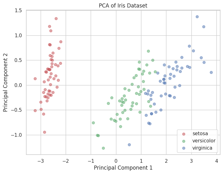
PCA is a dimensionality reduction technique that uses linear algebra concepts to project data onto principal components.

import numpy as np
import matplotlib.pyplot as plt
from sklearn.decomposition import PCA
from sklearn.datasets import load_iris

# Load dataset
iris = load_iris()
X = iris.data
y = iris.target

# Perform PCA
pca = PCA(n_components=2)
X_pca = pca.fit_transform(X)

# Plot the PCA result
plt.figure(figsize=(8, 6))
for target, color, label in zip([0, 1, 2], ['r', 'g', 'b'], iris.target_names):
    plt.scatter(X_pca[y == target, 0], X_pca[y == target, 1],
                color=color, label=label, alpha=0.5)
plt.xlabel('Principal Component 1')
plt.ylabel('Principal Component 2')
plt.title('PCA of Iris Dataset')
plt.legend()
plt.show()

Output:

10. 💡 Real-World Applications

💡 Recommendation Systems

Linear algebra is fundamental in building recommendation systems, particularly in matrix factorization techniques used by collaborative filtering.

Example: Matrix Factorization for Recommendations

import numpy as np
from sklearn.decomposition import TruncatedSVD

# Sample user-item rating matrix
R = np.array([[5, 3, 0, 1],
              [4, 0, 0, 1],
              [1, 1, 0, 5],
              [1, 0, 0, 4],
              [0, 1, 5, 4],
              [2, 1, 3, 0]])

# Perform SVD
svd = TruncatedSVD(n_components=2, random_state=42)
U = svd.fit_transform(R)
Sigma = svd.singular_values_
VT = svd.components_

# Reconstruct the approximate matrix
R_approx = np.dot(U, np.dot(np.diag(Sigma), VT))
print("Original Rating Matrix R:\n", R)
print("\nApproximated Rating Matrix R_approx:\n", R_approx)

Output:

Original Rating Matrix R:
 [[5 3 0 1]
 [4 0 0 1]
 [1 1 0 5]
 [1 0 0 4]
 [0 1 5 4]
 [2 1 3 0]]

Approximated Rating Matrix R_approx:
 [[4.82703214 2.69731693 1.65298163 1.23792399]
 [3.9475689  1.97553773 1.20528293 1.13632068]
 [1.52191034 1.20030495 2.3289128  4.45047898]
 [1.2822962  0.98632572 1.55765659 3.24249006]
 [0.58813405 1.27930172 4.02134715 3.23390214]
 [1.73707554 0.91936213 2.65541368 0.84254703]]

💡 Computer Vision

In computer vision, linear algebra is used for image transformations, feature extraction, and deep learning architectures.

Example: Image Rotation Using Matplotlib and NumPy

import numpy as np
import matplotlib.pyplot as plt
from scipy.ndimage import rotate
from skimage import data

# Load a sample image
image = data.camera()

# Rotate the image by 45 degrees
rotated_image = rotate(image, 45, reshape=True)

# Display original and rotated images
fig, axes = plt.subplots(1, 2, figsize=(12, 6))
axes[0].imshow(image, cmap='gray')
axes[0].set_title("Original Image")
axes[0].axis('off')

axes[1].imshow(rotated_image, cmap='gray')
axes[1].set_title("Rotated Image (45°)")
axes[1].axis('off')

plt.show()

Output:

💡 Natural Language Processing (NLP)

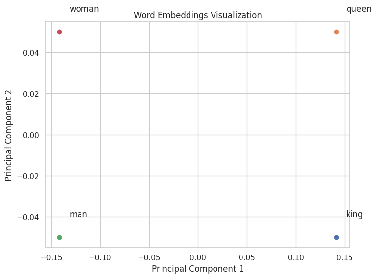
Linear algebra is employed in NLP for representing text data as vectors, such as in word embeddings and transformer models.

Example: Word Embeddings with NumPy

import numpy as np
import matplotlib.pyplot as plt
from sklearn.decomposition import PCA

# Sample word vectors (for demonstration purposes)
words = ['king', 'queen', 'man', 'woman']
vectors = np.array([
    [0.8, 0.6, 0.0],
    [0.8, 0.6, 0.1],
    [0.6, 0.8, 0.0],
    [0.6, 0.8, 0.1]
])

# Perform PCA to reduce to 2D
pca = PCA(n_components=2)
vectors_2d = pca.fit_transform(vectors)

# Plot the word vectors
plt.figure(figsize=(8, 6))
for i, word in enumerate(words):
    plt.scatter(vectors_2d[i, 0], vectors_2d[i, 1])
    plt.text(vectors_2d[i, 0]+0.01, vectors_2d[i, 1]+0.01, word)

plt.title("Word Embeddings Visualization")
plt.xlabel("Principal Component 1")
plt.ylabel("Principal Component 2")
plt.grid(True)
plt.show()

Output:

11. 💡 Machine Learning Integration

💡 Visualizing Model Performance

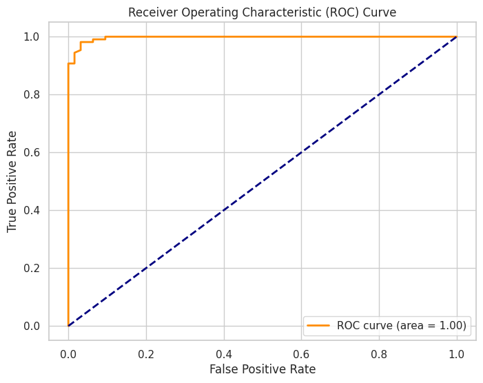
Data visualization is crucial for evaluating and interpreting machine learning models. It helps in assessing model accuracy, diagnosing issues, and comparing different models.

Example: ROC Curve

import matplotlib.pyplot as plt
import seaborn as sns
from sklearn.datasets import load_breast_cancer
from sklearn.model_selection import train_test_split
from sklearn.ensemble import RandomForestClassifier
from sklearn.metrics import roc_curve, auc

# Load dataset
data = load_breast_cancer()
X = data.data
y = data.target

# Split data
X_train, X_test, y_train, y_test = train_test_split(X, y, test_size=0.3, random_state=42)

# Train model
clf = RandomForestClassifier(n_estimators=100, random_state=42)
clf.fit(X_train, y_train)

# Predict probabilities
y_probs = clf.predict_proba(X_test)[:, 1]

# Compute ROC curve and AUC
fpr, tpr, thresholds = roc_curve(y_test, y_probs)
roc_auc = auc(fpr, tpr)

# Plot ROC curve
plt.figure(figsize=(8, 6))
plt.plot(fpr, tpr, color='darkorange',
         lw=2, label=f'ROC curve (area = {roc_auc:.2f})')
plt.plot([0, 1], [0, 1], color='navy', lw=2, linestyle='--')
plt.title('Receiver Operating Characteristic (ROC) Curve')
plt.xlabel('False Positive Rate')
plt.ylabel('True Positive Rate')
plt.legend(loc="lower right")
plt.show()

Output:

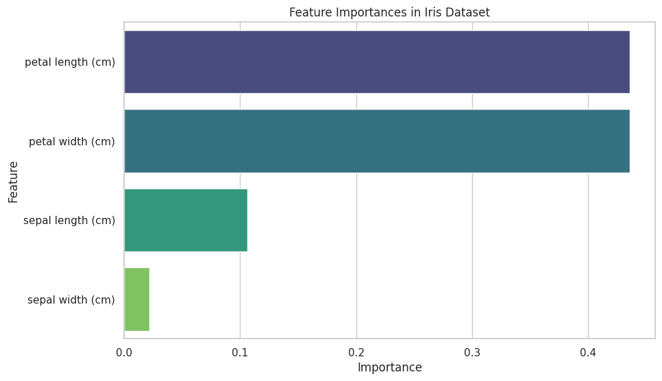
💡 Feature Importance Visualization

Understanding which features contribute most to your model's predictions can inform feature engineering and model interpretation.

Example: Feature Importance Plot

import matplotlib.pyplot as plt
import seaborn as sns
from sklearn.datasets import load_iris
from sklearn.ensemble import RandomForestClassifier
import pandas as pd
import numpy as np

# Load dataset
iris = load_iris()
X = iris.data
y = iris.target
feature_names = iris.feature_names

# Train model
clf = RandomForestClassifier(n_estimators=100, random_state=42)
clf.fit(X, y)

# Get feature importances
importances = clf.feature_importances_
features = pd.Series(importances, index=feature_names).sort_values(ascending=False)

# Plot feature importances
plt.figure(figsize=(10, 6))
sns.barplot(x=features.values, y=features.index, palette="viridis")

# Add title and labels
plt.title("Feature Importances in Iris Dataset")
plt.xlabel("Importance")
plt.ylabel("Feature")

# Show the plot
plt.show()

Output:

💡 Confusion Matrix Heatmap

A confusion matrix visualizes the performance of a classification model by showing the true vs. predicted classifications.

Example: Confusion Matrix Heatmap with Seaborn

import matplotlib.pyplot as plt
import seaborn as sns
from sklearn.metrics import confusion_matrix, classification_report
from sklearn.model_selection import train_test_split
from sklearn.ensemble import RandomForestClassifier
from sklearn.datasets import load_iris
import pandas as pd

# Load dataset
iris = load_iris()
X = iris.data
y = iris.target

# Split data
X_train, X_test, y_train, y_test = train_test_split(X, y, test_size=0.3, random_state=42)

# Train model
clf = RandomForestClassifier(n_estimators=100, random_state=42)
clf.fit(X_train, y_train)

# Predict
y_pred = clf.predict(X_test)

# Compute confusion matrix
cm = confusion_matrix(y_test, y_pred)
cm_df = pd.DataFrame(cm, index=iris.target_names, columns=iris.target_names)

# Create a heatmap
plt.figure(figsize=(8, 6))
sns.heatmap(cm_df, annot=True, cmap='Blues', fmt='d')

# Add title and labels
plt.title("Confusion Matrix of Random Forest Classifier")
plt.xlabel("Predicted Label")
plt.ylabel("True Label")

# Show the plot
plt.show()

# Print classification report
print(classification_report(y_test, y_pred, target_names=iris.target_names))

Output:

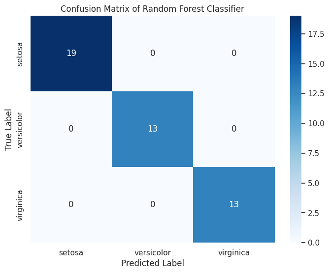
                precision    recall  f1-score   support

      setosa       1.00      1.00      1.00        19
  versicolor       1.00      1.00      1.00        13
   virginica       1.00      1.00      1.00        13

    accuracy                           1.00        45
   macro avg       1.00      1.00      1.00        45
weighted avg       1.00      1.00      1.00        45

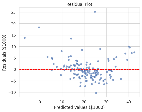
💡 Residual Plot for Regression Models

Residual plots help in diagnosing the performance of regression models by showing the difference between observed and predicted values.

Example: Residual Plot with Seaborn

import pandas as pd
import numpy as np
import matplotlib.pyplot as plt
import seaborn as sns
from sklearn.linear_model import LinearRegression
from sklearn.model_selection import train_test_split

# Load Boston dataset from original source
data_url = "http://lib.stat.cmu.edu/datasets/boston"
raw_df = pd.read_csv(data_url, sep="\s+", skiprows=22, header=None)

# Preprocess the dataset
data = np.hstack([raw_df.values[::2, :], raw_df.values[1::2, :2]])
target = raw_df.values[1::2, 2]

# Create a DataFrame for easier handling
feature_names = [
    "CRIM", "ZN", "INDUS", "CHAS", "NOX", "RM", "AGE", 
    "DIS", "RAD", "TAX", "PTRATIO", "B", "LSTAT"
]
boston_df = pd.DataFrame(data, columns=feature_names)
boston_df["PRICE"] = target

# Split data into features and target
X = boston_df.drop(columns=["PRICE"])
y = boston_df["PRICE"]

# Split data into training and testing sets
X_train, X_test, y_train, y_test = train_test_split(X, y, test_size=0.3, random_state=42)

# Train Linear Regression model
model = LinearRegression()
model.fit(X_train, y_train)

# Predict on test data
y_pred = model.predict(X_test)

# Calculate residuals
residuals = y_test - y_pred

# Create a residual plot
sns.scatterplot(x=y_pred, y=residuals, alpha=0.7)
plt.axhline(0, color='red', linestyle='--')

# Add title and labels
plt.title("Residual Plot")
plt.xlabel("Predicted Values ($1000)")
plt.ylabel("Residuals ($1000)")

# Show the plot
plt.show()

Output:

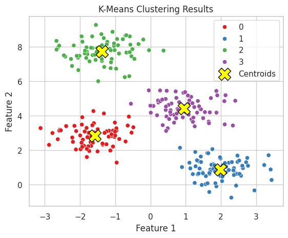
💡 Clustering Visualization

Visualizing clustering results helps in understanding the grouping and validating the clustering performance.

Example: K-Means Clustering Visualization

import matplotlib.pyplot as plt
import seaborn as sns
from sklearn.datasets import make_blobs
from sklearn.cluster import KMeans
from matplotlib.colors import ListedColormap
import pandas as pd
import numpy as np

# Generate synthetic data
X, y = make_blobs(n_samples=300, centers=4, cluster_std=0.60, random_state=0)
data = pd.DataFrame(X, columns=['Feature1', 'Feature2'])

# Perform K-Means clustering
kmeans = KMeans(n_clusters=4)
kmeans.fit(X)
data['Cluster'] = kmeans.labels_

# Create a scatter plot with clusters
sns.scatterplot(data=data, x='Feature1', y='Feature2', hue='Cluster', palette='Set1', legend='full')

# Plot cluster centers
plt.scatter(kmeans.cluster_centers_[:, 0], kmeans.cluster_centers_[:, 1],
            s=300, c='yellow', edgecolor='black', marker='X', label='Centroids')

# Add title and labels
plt.title("K-Means Clustering Results")
plt.xlabel("Feature 1")
plt.ylabel("Feature 2")
plt.legend()

# Show the plot
plt.show()

Output:

12. 💡 Conclusion

Linear algebra is the bedrock of many machine learning algorithms, from the simplest linear regression to complex deep learning models. By mastering vectors, matrices, and their operations, you gain the ability to understand and manipulate data at a fundamental level, optimize models efficiently, and implement advanced techniques like dimensionality reduction and matrix factorization. Continue practicing these concepts through coding exercises and real-world applications to solidify your understanding and enhance your machine learning proficiency. Keep pushing forward on your journey to becoming a Tensorflow boss!